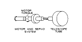
Figure 1. Simple model of antenna structure.
Keywords: Radio telescopes, antennas, servo system, pointing, structural
dynamics, offsetting.
Switching performance depends on the acceleration capacity, and on the dynamics of the servo and the antenna structure. For this application, the acceleration capacity as defined by the motor torque is not a limiting factor.
Hence, the servo dynamics and the antenna dynamics, and the interaction between the two, will determine the performance. The dynamics of the structure plays a role in two ways. Firstly, the part of the dynamics that is seen by the servo defines how the servo can be designed and which servo bandwidth that is achievable. Secondly, both the part that is visible and the part that is invisible to the servo respond to servo actions and perform ringing. Such ringing may influence pointing and image quality for a period of time after servo activity.
The present investigation has concentrated on the servo and its interaction
with the structural dynamics. For these effects, a reasonably simple model
of the antenna structure gives a good approximation to system performance.
The high order ringing effects are deferred to a separate study based on
a finite element model of the structure.
Figure 1. Simple model of antenna structure.
For simplicity, the model depicted in Figure 1 does not include a gear. It can easily be added without changing the principles. Alternatively, all moments of inertia and other parameters can be referred to the same axis. Also, viscous friction is not shown. For the first linear considerations, viscous friction proportional to angular velocity is assumed to exist between load and ground leading to a damping ratio of about 0.02. Non-linear bearing friction will be considered later.
From Newton's second law, it is straightforward to formulate the system
equations and to set up a block diagram of the system. A block diagram
of the structure can be seen in Figure 2. The input is electric torque
on the motor shaft. The motor velocity (~tachometer reading) or load position
(~encoder reading) would be typical interface points for the servo.
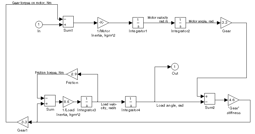
Figure 2. Block diagram of system schematically shown in Figure
1.
For the present configuration, the following values have been used:
| Motor inertia | 0.0091 | kgm2 |
| Load inertia | 117000 | kgm2 |
| Gear ratio | 3000 | |
| Series stiffness | 462 | MNm |
| Viscous friction | 294000 | Nms |
| L.r.r. frequency | 10 | Hz |
The considerations are equally valid for designs with one or two motors per axis. If two motors are used, the motor inertia refered to above should be replaced by the sum of the moments of inertia of the two motors. In addition, it should be ensured that oscillations of the two motors against each other would not pose problems. This is outside the scope of the present study.
The system is of fourth order. It has an eigenfrequency of 15.6 Hz and
two eigenvalues very close to zero, corresponding to free body motion.
An overwhelming part of the telescopes and radio telescopes in use today use cascade controllers. Attempts have been made to apply state space controllers but these appear not to have been successful. On the other hand, modern control theory has already for a long time been based on state-space techniques. Hence, it is expected that at some time in the future, reliable state-space controllers for astronomical telescopes will find widespread use. However, due to the limited success so far, it was found to be conservative to base the considerations on traditional cascade controllers.
The servo system for the antenna is shown in Figure 3. The drive has
torque motors with a current loop (not shown) to speed up the system by
reducing the effect of the inductance in the motor windings. There is a
tachometer loop with velocity feedback from the motor shafts. Experience
shows that velocity feedback should be taken from the motor shaft to avoid
stability problems from high-order resonances.
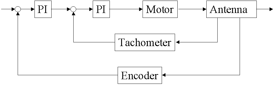
Figure 3. Overview of a conventional servo system for radio and optical telescopes. Compensation networks and current loop are not shown.
The encoder feedback should be taken as close as possible to the mechanical structure defining the antenna boresight, i.e. on the telescope tube (=load) of Figure 1. However, due to the distributed nature of the inertia, encoder feedback is in practice normally neither taken from the load nor the motor but rather "somewhere in between". This reflects the fact that the model shown in Figure 1 is highly simplified.
The tachometer and the position loops should be implemented digitally.
The sampling rate should be about 1 ms and this value is so high that the
system, for this introductory study, can be considered as continuous.
Figure 4 shows Bode plots for the tachometer loop. The solid curves
are open-loop Bode plots with appropriate scaling. It is essentially a
line falling 20 dB/decade because of the integrating effect of the motor.
At high frequencies, the motor and the load become decoupled. This is seen
as a decrease in inertia, and for high frequencies the amplitude ratio
line is located higher than for low frequencies. The phase never goes below
-90º and, ideally, any high bandwidth can be obtained even with a
simple P controller.
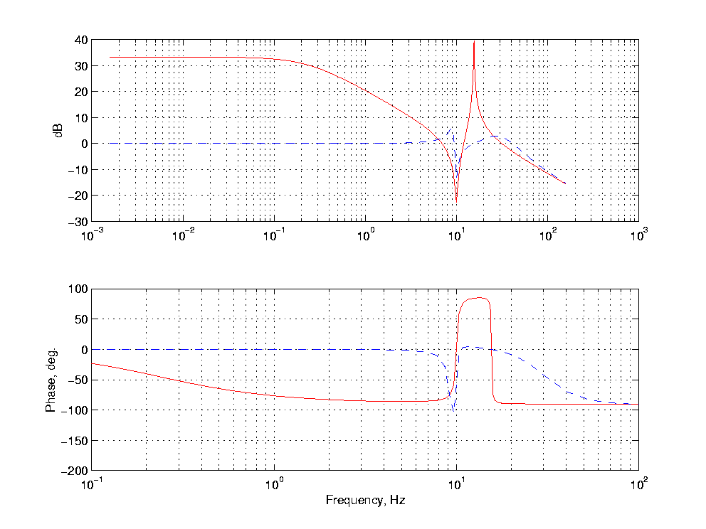
Figure 4. Bode plots for open and closed tacholoopes, repsectively.
The open loop curves are solid, and the closed loop dashed.
In practice, secondary resonances in the structure limit the bandwidth of the tacho loop. Experience shows that the bandwidth achievable depends on the ratio between the moment of inertia of the motor and the load, referred to the same axis. If the ratio is <<1, as for a direct drive, the bandwidth achievable is normally somewhat below the locked rotor resonance frequency. If the ratio is >>1, as for a small motor and a large gear ratio, a very high bandwidth above, say, 100 Hz is achievable.
For the present application, the ratio between the motor and load moments of inertia referred to the same axis is 0.7, i.e. close to a matched inertia condition. This is a value traditionally selected, partially for historical reasons. It corresponds to a matching of impedance in an electric network and is optimal from an energy transfer point of view. However, from a stabilization point of view it is unpleasant3.
From experience it is reasonable to expect a bandwidth of about 50 Hz for the present system but it would require a finite element analysis to give a more clear answer. For the present analysis, it has been assumed that a bandwidth of 50 Hz is obtainable. The break frequency of the PI has been chosen to be 30 Hz. For these choices, the closed loop bode plots are shown dashed in the curves. There is a dip near the locked rotor frequency, corresponding to a peak in the amplitude ratio for the load (not shown).
The open position loop is shown in Figure 5. The encoder signal is here
taken from the antenna load and not from the motor. Thus, the dip near
the locked rotor resonance frequency found in the tacho loop now appears
as a resonance peak. As for the velocity loop, the curve drops 20 dB/decade
at low frequencies.
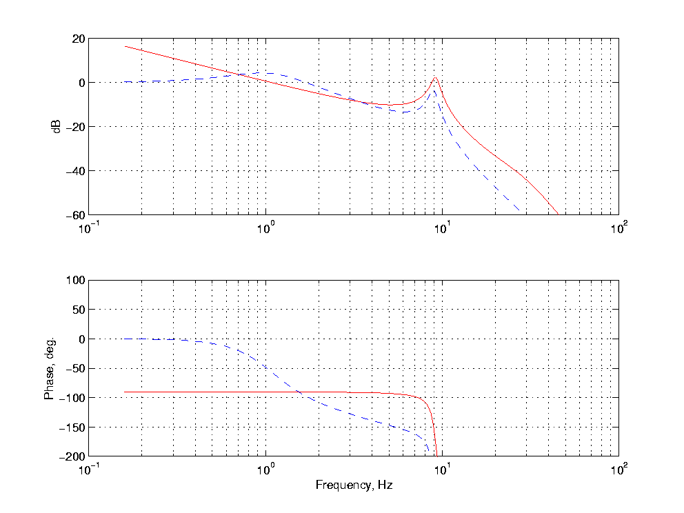
Figure 5. Open and closed loop frequency responses for the position
loop. Encoder feedback is taken from the load. The open loop responses
are solid and the closed loop plots dashed.
Due to the drastic phase shifts near the resonance peak, it is for this configuration, with conventional means, not possible to achieve bandwidths higher than 3-5 times below the locked rotor resonance frequency (10 Hz). For the present case, a PI controller with a break frequency of 0.8 Hz in series with a first-order lowpass filter with a break frequency of 4 Hz has been selected. This gives a closed loop bandwidth of about 2 Hz. The frequency response of the closed position loop is shown dashed in Figure 5.
If the encoder is connected to the motor shaft, it is possible to obtain
a faster servo system. The bandwidth can be 4-5 Hz. This is demonstrated
in Figure 6, showing open and closed position loop frequency responses
with encoder feedback from the motor.
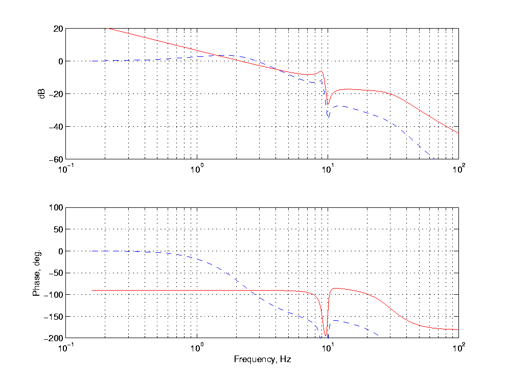
Figure 6. Open and closed loop frequency responses for the position
loop. Encoder feedback is taken from the motor shaft. The open loop responses
are solid and the closed loop plots dashed.
As mentioned before, in practice the encoder signal is neither taken from the motor shaft nor the load but rather somewhere in between. Hence, the two cases described constitute limit cases. It would take a more detailed model based on a finite element calculation to go into details.
In some cases it is necessary to force the bandwidth of the position
loop to a value near or above the locked rotor resonance frequency. The
remedy for this is to insert a notch filter in series with the controller.
In this way, it is, in principle, possible to cancel resonance effects
near the locked rotor resonance frequency. However, in practice this approach
is often dangerous, in particular for physically large systems. Such a
system can be highly susceptible to parameter changes causing drift, and
the risk of instability is high. Also, for the azimuth movement, corrections
must be made for parameter changes due to change in elevation angles. Hence
this approach is not attractive for general use.
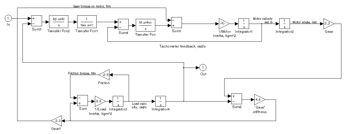
Figure 7. Block diagram of complete, linear model applied for this
study. The diagram is shown with poision feedback from the load. Alternatively,
the feedback can be taken from the motor shaft.
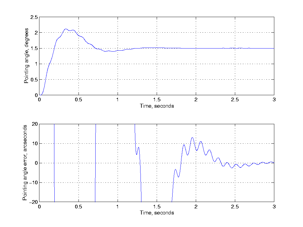
Figure 8. Step response of complete system. Encoder feedback is
here taken from the load. It can be seen that the system is inherently
too slow and that ringing is not critical.
Although some "ringing" occurs, the step response shows that the major problem in this configuration is the low bandwidth of the position loop. On the other hand, the bandwidth would need an improvement of only a factor about 1.5. This is roughly the uncertainty in the servo system design of this study. Hence, system performance is marginal and it would take a more detailed study to determine whether the specification can be met.
It can also be seen that with position feedback from the load, ringing may not be a problem.
For the configuration where the position feedback is taken from the motor, the step responses shown in Figure 9 are obtained. The system is now faster than for Figure 8 but heavy ringing takes place due to the fact that the load movement is outside the servo loop.
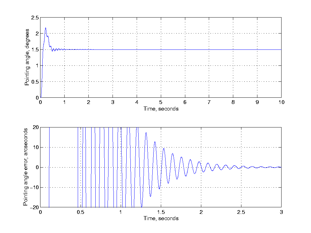
Figure 9. Step responses for a system with position feedback from
the motor. The curves above show the movement of the load. Intense ringing
occurs.
Two approaches can be identified. The first is to change the system dynamics actively or passively. One or more damping loops can be added. This can be accomplished using observers to identify the unmeasured states or by adding load feedback from accelerometers. Such an approach has been used for some optical telescopes1,4 but may not be attractive for the present application due to its complexity.
The other method is to apply special shaped inputs to avoid or suppress ringing. There are important applications for this approach within the fields of hard disk drives and spacecraft orientation mechanisms. Hence, a considerable amount of research has been done within this area.
The simplest shaped input techniques merely apply smooth curves. For optical telescopes it has for some time been general practice to round the corners of the input trajectories using polynomia. Von Hoerner has proposed half sine waves to accomplish the same5. Other methods apply input trajectories with only little power at the locked rotor resonance frequency 6,7,8,9,10.
The most promising method seems to be the approaches that first excite
ringing and secondly cancels it11,12,13,14,15. For a single
oscillation mode, as assumed in this context, the approach simply subdivides
a step into two. The first step excites the vibration and the second one
cancels it. This can be seen in Figure 10 that is based upon an input shape
as shown in Figure 11. In practice the method is somewhat more complex
since ringing may occur at more than one frequency.
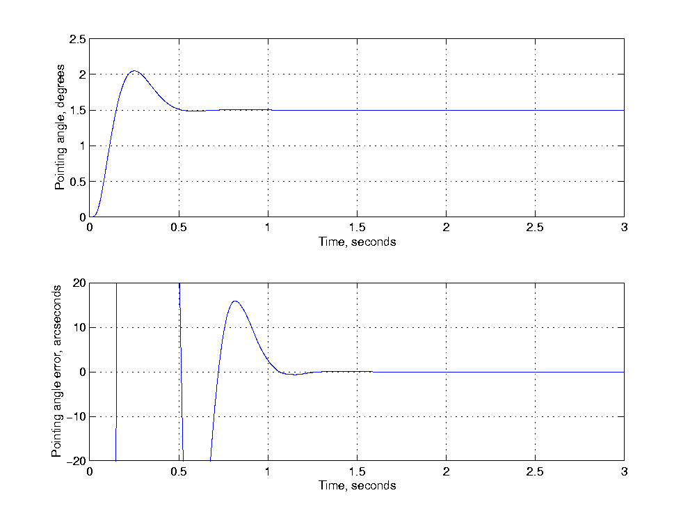
Figure 10. Step responses fro a system with position feedback from
the motor. The curves above show the movement of the load. The input curve
is shown in Figure 11. Ringing is completely avoided.
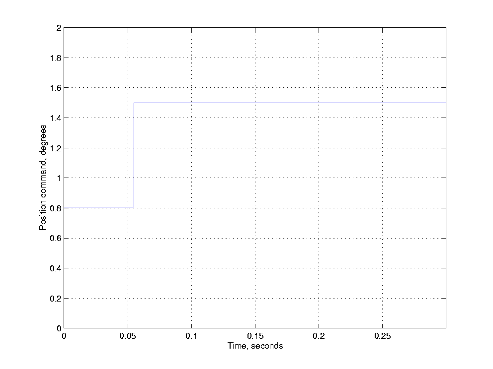
Figure 11. Shaped input curve applied to the position loop for the
step responses in Figure 10.
Shaped inputs may be applied in a feedforward mode, i.e. matching input curves may be applied simultaneously for both torque, velocity and position. This approach has not been investigated in great detail yet. However, it seems promising since the filtering effect of the slow position loop is avoided.
To demonstrate the potential of such an approach, shaped input curves as shown in Figure 12 have been generated. The position loop of the system was opened and the shaped velocity reference curve was used as input to the tachometer loop. Since the tachometer loop has a high bandwidth, it is possible to move the antenna quickly.
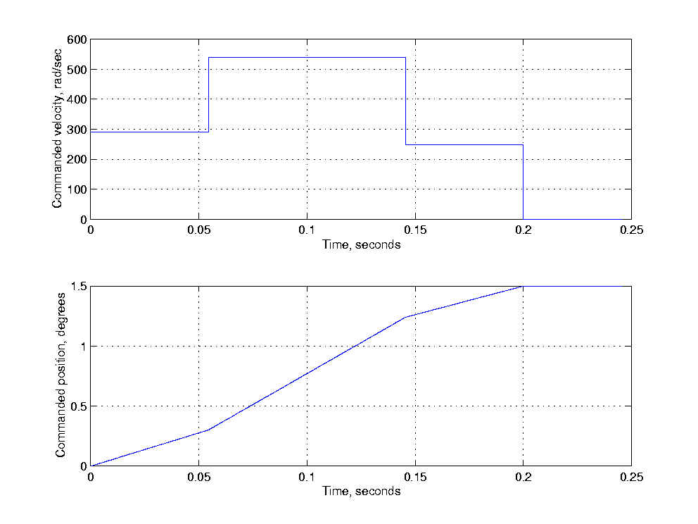
Figure 12. Shaped input vurves for velocity (top) and position (bottom).
The resulting trajectory is seen in Figure 13. It is seen that the antenna
moves 1.5 degrees within about 200 ms. Although there will be other limiting
factors not included in the model (such as tachometer errors and secondary
resonances), these curves indicate that a combination of shaped inputs
with feedforward techniques has a high potential and should be studied
further.
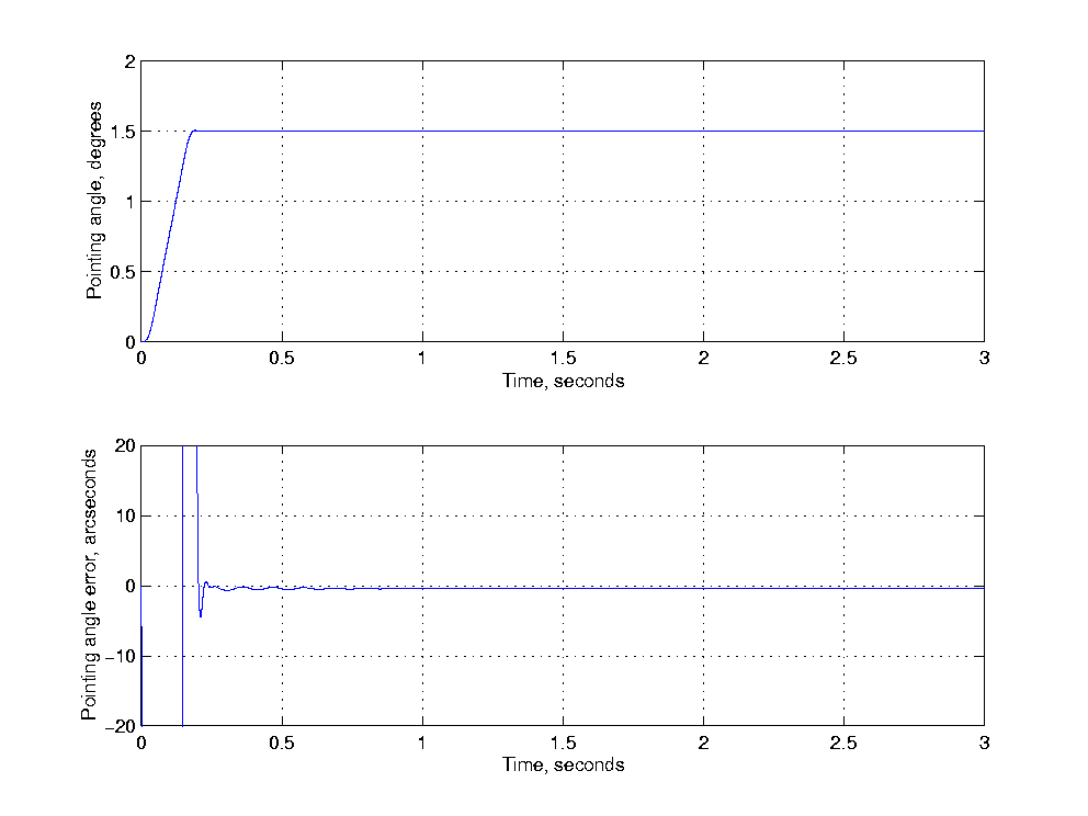
Figure 13. Responses for a system with tachometer loop only. The
velocity profile of Figure 12 has been applied as input. The upper curve
is load position from which the poistion profile of the lower curve of
Figure 12 has been subtracted and appropriately scaled. No ringing occurs
in spite of the short transition time.
2 Andersen, T.: The Servo System of the EISCAT Svalbard Antenna. Proc. SPIE, Vol. 2479, pp. 301-312. April 19-21, 1995.
3 Wilson, D.R. & M.M. Butler: Compensation of Servodrive Resonances. Proc. IEE, Vol. 119, No. 10, pp. 1517-1520. October 1972.
4 Andersen, T.: Design of CAT Main Servos. European Southern Observatory Note EG-78/02, March 13, 1978.
5 von Hoerner, S.: Preventing Oscillations of Large Radio Telescopes after a Fast Stop. GBT Memo 152, June 1996.
6 Holdaway, M.A.: Elevation Dependence in Fast Switching. MMA Memo 221, July 13, 1998, describing method by David Woody.
7 Meckl, P.H. & W.P. Seering: Shaping Reference Inputs to Reduce Residual Vibration for a Cartesian Robot. pp. 225-240. Source unknown.
8 Aspinwall, D.M.: Acceleration Profiles for Minimizing Residual Response. Journal of Dynamic Systems, Measurement, and Control, vol. 102, pp. 3-6, March 1980.
9 Meckl, H. & W.P. Seering: Reducing Residual Vibration in Systems with Time-Varying Resonances. Proc. International Conf. on Robotics an Automation, IEEE, 1987, pp. 1690-1695.
10 Yamamura,H., K. Ono, and M. Nishimura: Vibrationless Acceleration Control of Positioning Mechanisms and its Applications to Hard Disk Drives. Proc. of the International Conference on Advanced Mechatronics, Tolyo, Japan, May 21, 1989, pp. 25-30.
11 Swigert, C.J.: Shaped Torque Techniques. J. Guidance and Control, vol. 3, no 5, p. 460-467, Sept.-Oct. 1980.
12 Bhat, S.P. & D.K. Miu: Precise Point-to-Point Positioning Control of Flexible Structures. Journal of Dynamic Systems, Measurement and Control. Trans. ASME, vol. 112, Dec. 1990, pp. 667-674.
13 Sato, O., H. Shimojima & T. Kaneko: Positioning Control of a Gear Train System Including Flexible Shafts. JSME International Journal, vol. 30, No. 267, pp. 1465-1472.
14 Kuo, C.F. & C.Y. Kuo: Efficient Control of a Flexible Robot Arm by Shaped Inputs. DSC-Vol. 38, Adctive Control of Noise and Vibration, ASME 1992, pp. 261-270.