ABSTRACT

Imaging simulations have been carried out with a version of the spiral zoom array presented in Conway(2000) (Memo 283). Two test images were used, one based on a VLA image of Cygnus A and another based on an OVRO CO map of M51. Both snapshot and long track CLEAN simulations were carried out. The results were compared with those obtained for a single ring array with similar resolution. The single ring array has a fairly uniform coverage out to its maximum baseline and therefore provides a useful constrast to the spiral zoom array which has a strongly tapered (almost gaussian) coverage. For both test images the spiral array gave better imaging performance. The difference was particularly large for the case of the long-track observations when the rms errors were 10 times larger for the ring than for the spiral arrays. This large difference arises because the large near-in sidelobes of ring arrays, caused by the sharp edge to the uv-coverage, persists even after a long track.

These simulations illustrate that it is important to consider that deconvolution requires both extrapolation of the uv data as well as interpolation between uv points. A naturally tapered uv coverage appears to provide more constraints on the necessary extrapolation than for the case of ring arrays. More imaging simulations must be carried out, paricularly comparing zoom arrays to the somewhat tapered 'donut' or 'double ring' arrays that have been proposed. However, these intial tests show that spiral zoom arrays have good imaging performance as well as high observing efficiency (Conway 2000, Memo 283) and the ability to have finely adjustable resolution (Conway 1998, Memo 216).

1. INTRODUCTION

To test the imaging performance of spiral zoom arrays, some snapshot and long track imaging simulations have been carried out. Two test images were used, one based on a VLA Cygnus A image (R.Perley & C.Carilli) and the other on an OVRO CO image of M51 (kindly donated by Susanne Aalto). The imaging performance has been compared with that of a 'generic' single ring array having the same resolution.

2. SPIRAL ARRAY

The spiral array tested was based on that presented in Conway(2000), ALMA Memo 283. Almost the same arrangement of pad positions were used. We chose to simulate the case when the telescopes were arranged in their largest spiral-like configuration. This array gives a resolution of 0.135 arcsec at 230GHz. For higher resolutions the telescopes can be mostly place on a 3km diameter outer ring (see memo 283, Fig 1 top). For smaller resolutions the antennas are placed in smaller spiral configurations which should have similar imaging performance to the array tested. The imaging tests here therefore are a general test of the imaging performance of a spiral geometry.

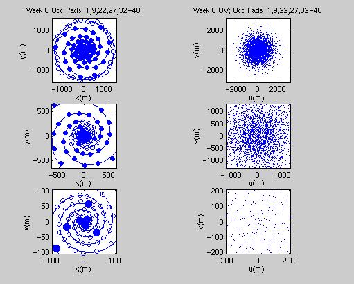
In the array tested the occupied pads on each arm are numbers 32 to 48, (see memo 283 for the numbering definition) and in addition pads 1,9,22 and 27, which is slightly different than in memo 283. Occupying these lower numbered pads improves the short spacing coverage of the array, and samples baselines down to 1.2 antenna diameters. As the array zooms inwards and antennas are taken from the largest pad numbers to fill up the lower numbered unoccupied pads (see Memo 283), but pads 1,9,22 and 27 remain occupied. Links to the antenna coordinates for this spiral array in UVCON format are given in the Appendix.

Note that to improve mosaicing preformance it might be advantagous to replace the 4 inner 12m telescopes (those on pad 1 of each arm and at the centre) with an array of 16 to 25 smaller (e.g 6m) dishes (Wright 1999, Memo 272).

3. RING ARRAY

The comparison ring array was chosen to have the same resolution of as the spiral at 230GHz. This is found to occur when it has a diameter of around 1500m (i.e. half the total size of the spiral arrays). Antennas were initially place evenly around the ring and were then perturbed in azimuth and radius by gaussian noise with sigma 0.05 radians and 0.05 of the radius respectively. This procedure was needed to remove ring and spike-like structure in the uv coverage of the perfectly regular ring arrays.

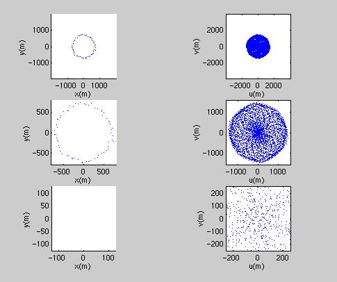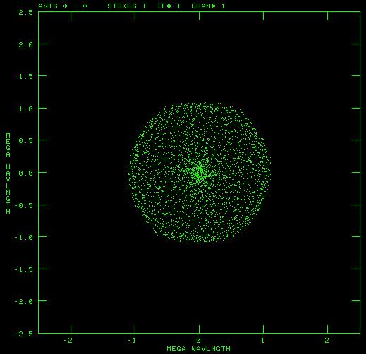
4. UV COVERAGES

Below are shown the zenith snapshot and long track uv coverage for the spiral and ring arrays respectively. The declination for the long track simulation was taken as -23 degrees and lasted for +/- 3hrs around transit.

Spiral-Array Zenith Snapshot	Spiral-Array 6hr Track (Dec = -23)

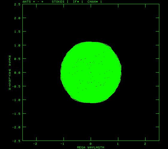Ring-Array Zenith Snapshot	Ring-Array 6hr Track (dec = -23)

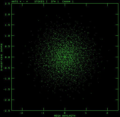
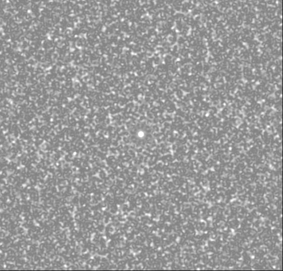
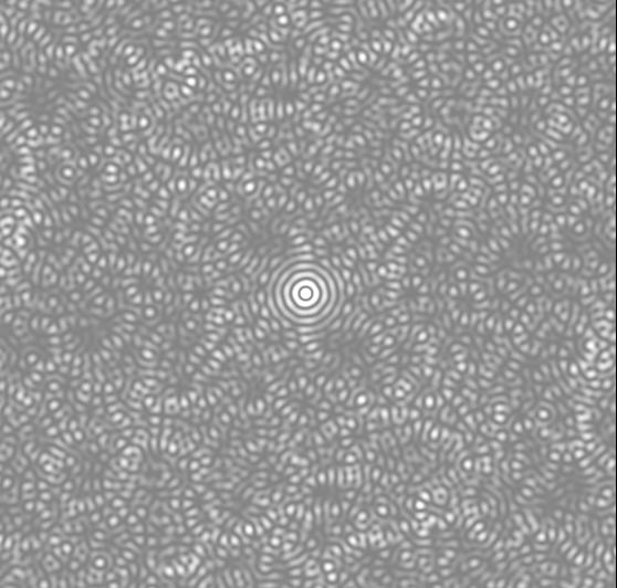
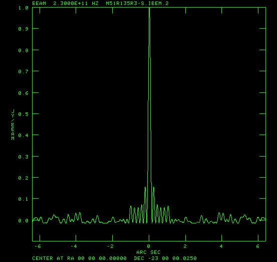
5. DIRTY BEAMS

Dirty beams were calculated assuming pure natural weighting (UVWTFN='NA', ROBUST=5). The cellspacing was 25mas, and the images below are 512 pixels square. For the long tracks it was assumed that all uv points had the same data weight with no account taken for increased noise as a function of elevation.

The resolution for the snapshots found from fitting the main lobe with a gaussian were 135mas FWHM circular for both the ring and spiral arrays. For the long track observations the FWHM increased slightly in the East-West direction to be 146mas for the spiral and 148mas for the ring. The small increase in resolution is what is expected if one considers the long track dirty beam as the linear sum of snapshot beams at each integration, these being in turn versions of the zenith snapshot beam rotated and stretched in one direction. Since the minimum elevation for the long track is around el_min= 45 degrees the stretching for the long track beam is order half of 1/sin(el_min).

While it is true that in centrally condensed uv coverages, such as those from a spiral array, uv points from subsequent integrations are very close together; the increase in the ratio of densities in the inner and outer parts of the uv plane is only a weak function of the length of the experiment if low elevations (<30 degrees) are avoided. To see this consider an array at the South pole having a uv coverage which is two rings observing a source at the South pole.

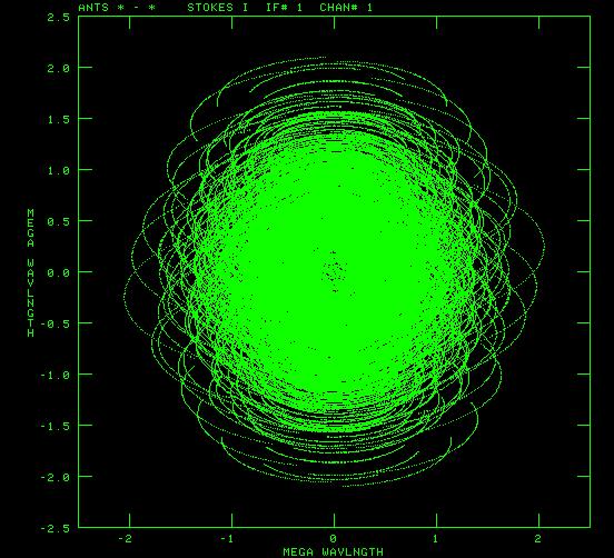
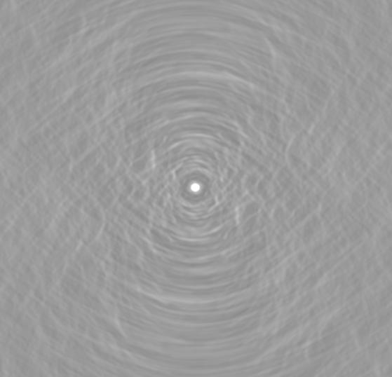
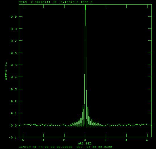
Note below the large ringlobes for the ring array (see Figs 4,5, bottom). In the North-South direction these sidelobe do not decrease significantly even for a long track (see Figs 4,5, bottom right), this is because they are due to the sharp edge to the uv coverage. In contrast because it is highly tapered even the spiral snapshot beam has very small near-in sidelobes, and only the occasional random peaks in the snapshot beam (see Fig 4, top left). As we go to long tracks the spiral array sidelobes decrease significantly in contrast to the case of ring arrays where the peak sidelobe remains at about 15% of the main lobe.

Spiral-Array Snapshot	Spiral-Array 6hr Track

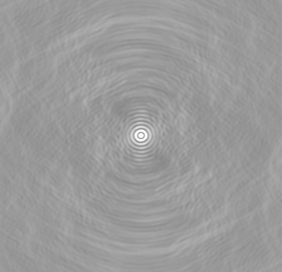Ring-Array Zenith Snapshot	Ring-Array 6hr Track

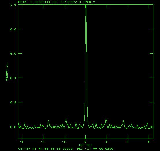
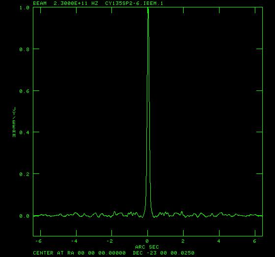
6. DIRTY BEAM SLICES (click for higher resolution)

Spiral-Array Zenith Snapshot	Spiral-Array 6hr Track

Ring-Array Zenith Snapshot	Ring-Array 6hr Track

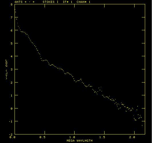
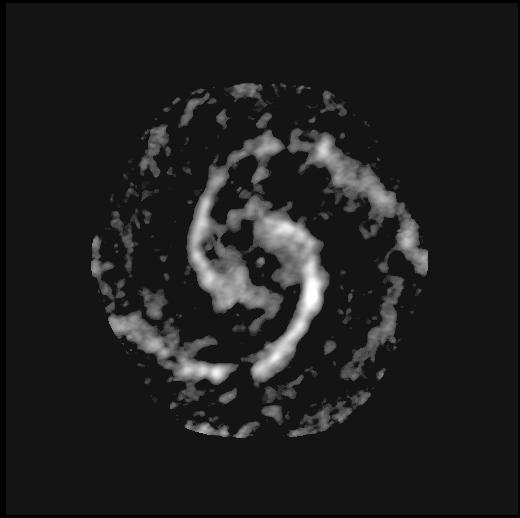
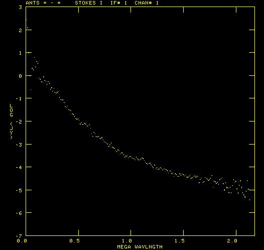
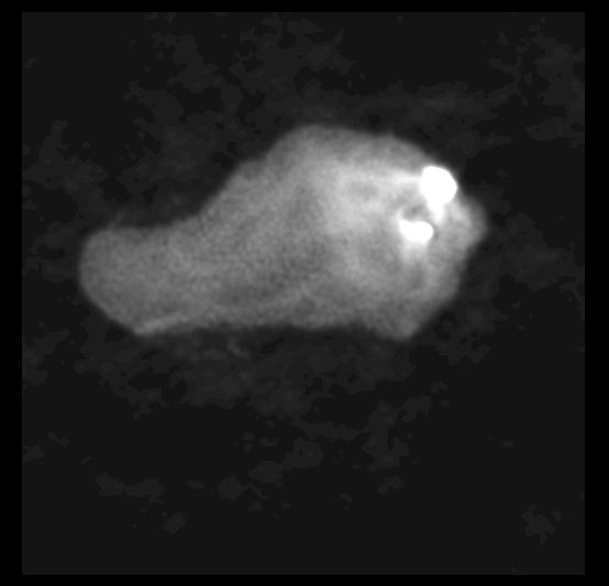
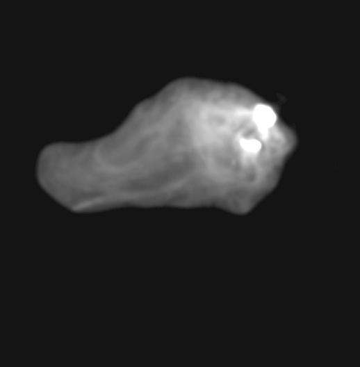
7. TEST IMAGES

Two test images were used in the simulations. One is based on a VLA image of one lobe of Cygnus A (Perley, Carilli et al) and one is based on an OVRO CO image of M51. Below are the images, and the falloffs of Log amplitude with uv distance they exhibit. The images have cellspacing of 25mas and sizes of 512 pixels square. The map units are in Jy/pixel, so they are considered as the true brightness distributions of the test sources and not to be convolved with any restoring beam. FITS versions of the test images can be obtained by ftp (see Appendix).

Cygnus A image	Cygnus A, Log Amp vs uv distance

M51 Image	M51, Log amp vs uv

8. IMAGING SIMULATIONS

Imaging simulations were carried out for the above two test images for ring and spiral arrays for both snapshots and long tracks. In each case noiseless data was created using AIPS task UVCON, using the arrays described in Sections 2 and 3 and assuming the observing frequency was 230GHz.

CLEAN deconvolution were performed using IMAGR, pure natural weighting, with 20,000 iterations for the snapshots and 50,000 for the long tracks. MINIPATCH=201 pixels, gain=0.1. The images were made 1024 pixels square with 25mas cellspacing but only the inner quarter of each dirty image was cleaned. All images were restored with a circular beam of FWHM 135mas. Finally error images were formed by subtracting a version of the true image convolved to 135mas resolution.

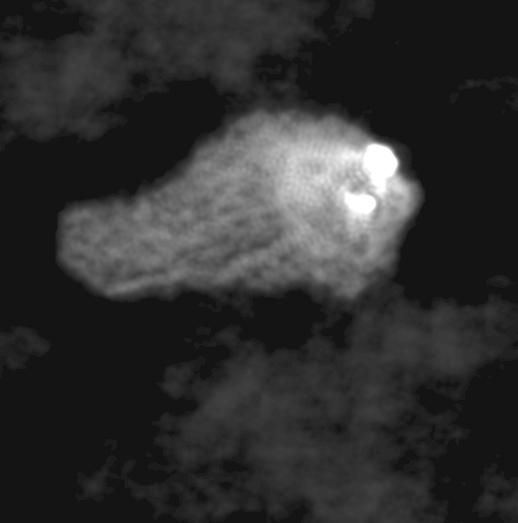
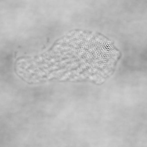
8.1. CYGNUS A - SNAPSHOT SIMULATIONS (Click Images for details)

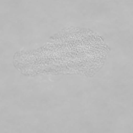Spiral-Array Image	Spiral-Array Errors

Ring-Array Images	Ring-Array Errors

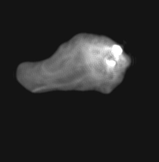
8.2. CYGNUS A - LONG TRACK SIMULATIONS (Click Images for detail)

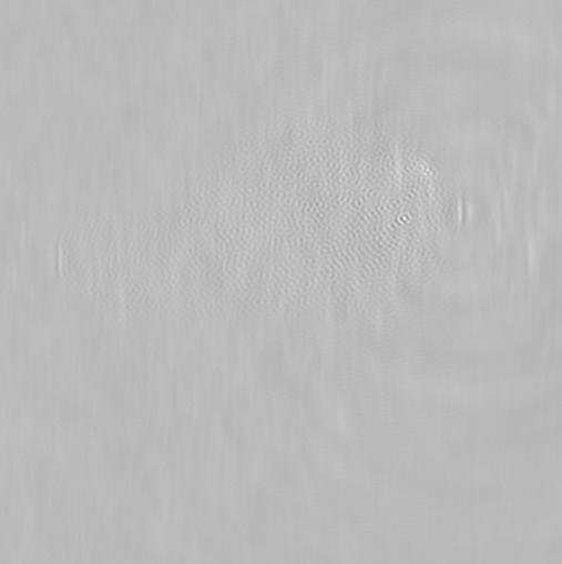Spiral-Array Image	Spiral-Array Errors

Ring-Array Image	Ring-Array Errors

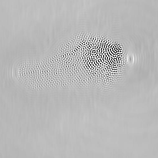
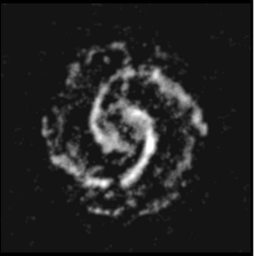
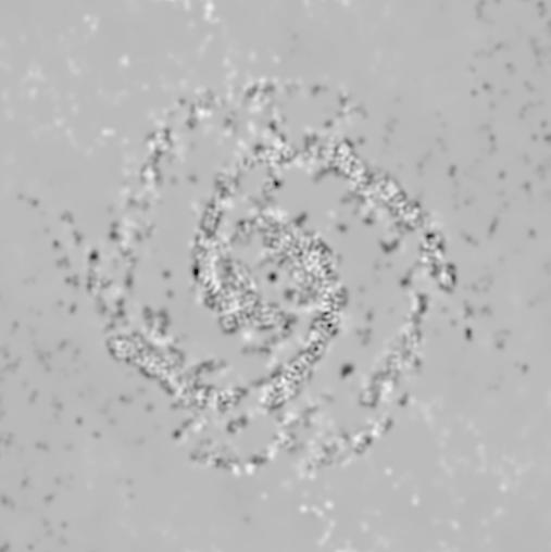
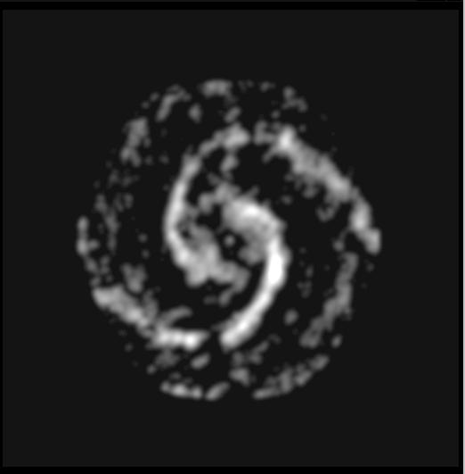
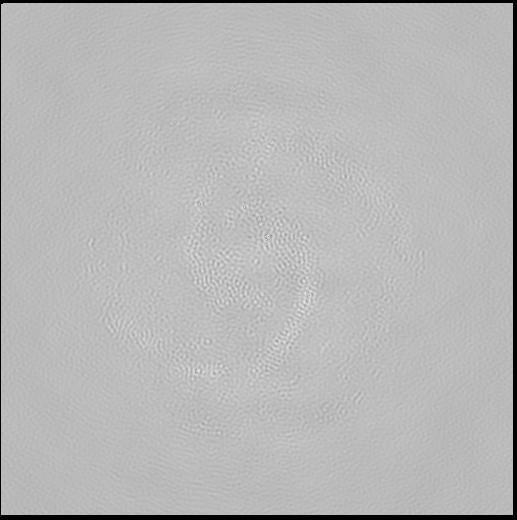
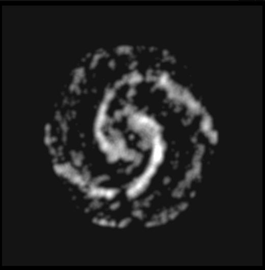
8.3. M51 - SNAPSHOT SIMULATIONS

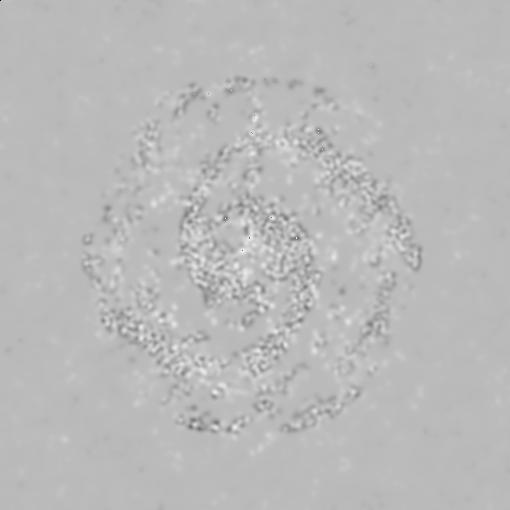Spiral-Array Image	Spiral-Array Errors

Ring-Array Image	Ring-Array Errors

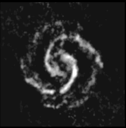
8.4. M51 - LONG TRACK SIMULATIONS

Spiral-Array Image	Spiral-Array Errors

Ring-Array Images	Ring-Array Errors

9. DISCUSSION

The simulations above show that, at least for the two test images used, the spiral array gave significantly better image reconstructions than the ring array, both for snapshots and for long tracks. For Cygnus A snapshots for instance (see Figure 7) the rms error was a factor of 2.02 less for the spiral than when using the ring arrays. The difference was even more dramatic for the long track simulations (see Figure 8) in which the spiral array rms error was better than that for the ring by a factor of 13.23. For the M51 test image (see Figures 9 and 10) the ring had rms errors larger than the spiral by factors of 1.47 and 13.85 for the snapshots and long tracks respectively.

The reason for the superior imaging performance of the spiral array is that the uv coverage is highly tapered. The sharp edge to the uv coverage which occurs for ring arrays and gives large systematic near-in sidelobes is therefore avoided. As shown in section 5, for ring arrays these large sidelobes persist even in the case of long track observations. It is clear that the dominant contributions to the error images for the ring array reconstructions (see Figures 7 to 10) are all ripple-like errors having a wavelength equal to the spacing of the near-in sidelobes.

In going from the dirty map to a more realistic estimate of the sky brightness distribution, deconcolution algorithms can be thought of as generating estimates of the visibility in regions which have not been measured. This is clear if one considers that the Fourier transform of the CLEAN or MEM map is in general not zero in unsampled parts of the uv plane, while in contrast the Fourier transform of the dirty map is by definition zero in these regions. As a aside to this, it follows that useful deconvolution algorithms which generates new visibilities estimates must be non-linear functions F of the dirty map in the sense that F(I1(x,y) + I2(x,y)) does not equal F(I1(x,y)) + F(I2(x,y)) where I1(x,y) and I2(x,y) are dirty maps.

The visibilities that CLEAN, MEM or some other non-linear algorithms must estimate which lie within the outer boundary of the uv coverage we can call interpolations while those beyond the edge of the uv coverage we can call extrapolations . In going from the dirty map to a better estimate it is clear that the deconvolution algorithms must both interpolate and extrapolate. The extrapolation property is needed to remove the large near-in sidelobes which arise from the sharp edge to the uv coverage. While A priori information such as positivity and limited-support can greatly help the process of interpolation between uv points it provides little help in doing the necessary extrapolation (which is effectively super-resolution). Ring-like arrays may be attractive in providing uniform and even complete (e.g Woody 1999, ALMA memo 270) uv coverage within circular regions but they have a large and probably unacceptable cost since they provide little aid in achieving the necessary uv extrapolation. The only way to avoid this problem for such arrays is to heavily taper the data. Such tapering is very expensive in lost sensitivity, since in order to reduce the near-in sidelobe level to that obtained by condensed arrays approximately 3/4 of the data has to be heavily tapered, decreasing sensitivity (and resolution) by of order a factor of 2.

In contrast the centrally condensed uv coverages such as that provided by spiral zoom arrays can be thought of (Conway 1998, ALMA Memo 216) as providing a dense well sampled core uv coverage plus outlier points. These outliers strongly constrain the extrapolation of the model to high spatial frequencies. One argument that is sometimes made for a uniform uv coverage within a circular boundary versus condensed is the analogy with an optical telescope such as the HST. In fact of course the effective uv coverage in this case is the autocorrelation of the circular aperture and is therefore in fact highly tapered. This high degree of tapering is one reason that deconvolution is rarely needed for the HST and points to having a similar condensed uv coverage for ALMA.

It will be interesting to compare the imaging performance of other types of arrays with spirals, particularly the minimum sidelobe arrays of Kogan. These of course minimise the largest sidelobe anywhere within the dirty beam while the gaussian-like uv coverages of spiral arrays effectively minimise the near-in sidelobes. The resulting uv coverages for the minimum sidelobe arrays (see memos 212, 217, 226) are intermediate in their natural tapering between single ring and spiral arrays, and have significantly reduced near-in sidelobes compared to pure rings. However the minimisation routine effectively concentrates on reducing the far sidelobes once the near-in sidelobes have been reduced below about 0.1. It seems likely that not all sidelobes are equally important for improving imaging and so reducing the systematic near-in sidelobes is probably more effective in removing ripple-like artifacts.

This memo suggests that at least for some classes of images spiral zoom arrays have superior imaging properties in addition to their advantages in array operating efficiency, construction and operating cost and tapering properties discussed in Conway(2000) (ALMA Memo 283). This present memo of course has only looked at two test images, and a wider range of simulations should be carried out before final conclusions can be drawn about imaging properties. It will be particularly interesting to study the multi-pointing (mosaicing) imaging capabilities of the array. In addition all of the simulations here used CLEAN, other deconvolution algorithms such as MEM might be worth trying; although MEM is notorious for leaving beam patterns embedded in extended structure and probably would not much help the Cygnus A reconstructions. Links to the coordinates of the antennas used in the spiral array presented in this memo are in UVCON format are given in the appendix below for anyone who wants to do their own imaging simulations with this array.

APPENDIX - TEST DATA

The UVCON format data for the spiral array used in this memo can be found at http://www.oso.chalmers.se/~jconway/ALMA/ARRAYS/ under the file name SP32T48-1-9-22-27.UVCON.

In addition FITS versions of the test images used in this memo can be found at http://www.oso.chalmers.se/~jconway/ALMA/IMAGES/ under filenames CYGCW5.SUBIM and M51OV2.IMG. Versions of rhese model images convolved with a restoring beam of 135mas can also be found in the same directory.