ALMA Memo No 348
A Preliminary ALMA Zoom Array Design
for the Chanjnantor Site.
John Conway
Onsala Space Observatory, Sweden
February 15th, 2001
Abstract
I present a preliminary zoom array design for ALMA fitted into the the
Chajnantor site, and compare its properties with the proposed double ring
strawperson array. Both arrays have virtually the same number of pads and
require almost the same number of antenna moves. To first order the two
arrays are shown to have similar radial distributions of baselines, although
the coverage of the zoom array is smoother and is slightly more centrally
condensed. For snapshots the peak sidelobes for the two styles of array are
similar. However the zoom array has 40% smaller peak sidelobes for long track
observations. For both snapshots and long tracks the degree of uv cell
occupancy for the two arrays is very similar. We argue that zoom arrays
will have slightly smaller or equal phase noise effects than dual ring arrays
of the same resolution. For the zoom array we show that North-South extended
array configurations with low sidelobes exist for observing Northern hemisphere
or South polar sources.
The zoom array is a very flexible design, which can accommodate many different
modes of operation. It can for instance be operated as set of fixed arrays like
the double ring, with the important difference that the sizes and numbers of
configurations are variable. Alternatively the array could be operated in a
continuous reconfiguration mode with perhaps six antennas being moved per week.
This mode of operation has some astronomical advantages and significant operational
advantages. However the array is operated, if antenna moves are prevented by
bad weather, the zoom array is always left in a configuration with a good uv
coverage without stranded 'outlier' antennas.
After a certain amount of convergence the two styles of array proposed for the
intermediate configurations are no longer dramatically different. However in
almost all performance areas we argue that the zoom array is slightly
superior. This combined with its much greater flexibility suggests that
the zoom array design should be chosen for the intermediate configurations. Put
another way - we find no strong argument in favour of (and several
against) building particular scale lengths into the array design as is
done in the dual ring design.
CONTENTS
1. Introduction:
2. Zoom Array Design:
2.1 Intermediate Spiral:
2.2 Compact Array:
2.3 Outer Ring:
2.4 Sidelobe Optimisation:
3. Array Description:
3.1 A-Array Equivalent:
3.2 B-Array Equivalent:
3.3 B/C-Hybrid Array:
3.4 C-Array Equivalent:
3.5 D-Array Equivalent:
3.6 E-Array Equivalent:
4. Comparisons with Double Ring Array: UV Coverages and Beams
4.1 Snapshot UV density distribution
4.2 Snapshot UV coverages and Dirty Beams
4.3 Long track uv densities
4.4 Long track dirty beams
4.4 Imaging Simulations
5. Comparisons with Double Ring Array: Operational
5.1 Array Flexibility
5.2 Operational Issues
5.3 Hybrid Arrays
5.4 Fitting the array into the Site.
5.5 Roads and Conduits.
5.6 Combined Array Imaging
5.7 Mosaicing
5.8 Pointing Errors
5.9 Phase Noise
5.10 Tapering.
5.11 Inverse Tapering and Super-resolution
6. Summary
7. Future Work
1. Introduction:
A number of recent memos have discussed possible ALMA array
configurations. For the best possible imaging
certain properties are clearly desirable including 1)
low sidelobes for snapshot and synthesised beams. 2) Good uniform
filling of the uv plane and 3) A wide range of sampled baseline lengths.
Unfortunately to some extent these properties
are mutually inconsistent which makes the optimisation problem
poorly defined. In addition there are important
practical and operational constraints. For ALMA as with any other
array these constraints are likely to play a deciding rule
in the array geometry. Amongst the constraints are that
the array must fit into the available terrain and that it should
minimise construction and operations costs. These goals
can be achieved by sharing as many pads between different
configurations as possible. Such pad sharing both minimises the
antenna pads and other infrastructure to be constructed and
minimises the number of antenna moves needed to go through
all configurations
Motivated primarily by the need to minimise infrastructure
requirements Conway(1998, memo 216)
proposed an array design on a self-similar
three armed spiral pattern. In addition to its high degree
of pad re-use it was found that this array had excellent uv
coverage properties. By a remarkable coincidence for certain
spiral parameters the snapshot uv coverage was found to have
a distribution close to Gaussian. Similar
zoom concepts were developed independently by Webster(1998, memo 233)
who noted that any continuously scalable array must have a
pad density distribution which scales as 1/r^{2}. It was
argued by Conway(1999, memo 260) that an initial generating geometry
based on a spiral pattern had advantages compared to
other 1/r^{2} generating distributions such as multiple
nested circles or random distributions.
Both Conway(1998, memo 216) and Webster(1998, memo 233) noted that the
continuous self-similarity property of a zoom array allowed
it to be operated in a wide range of operational modes. It could
for instance be operated as a set of conventional fixed
configurations or alternatively in a continuous 'zoom' mode.
In this second mode a few antennas are moved every few
days
and the array would gradually change in resolution. Comparisons
of the relative efficiencies of continuous and conventional
'burst' reconfiguration showed that that the continuous mode
could in fact be slightly more efficient (Guilloteau 1999, memo 274, Yun
1999, memo 277, and Conway 2000a, memo 283). A first attempt was made by
Conway(2000c, memo 292) to fit a zoom spiral array into the Chanjantor site;
this early sketch we will refer to as the 'zoom1' design.
This present memo present a more complete ('zoom2')
design. Specifically it has parameters, including the positioning
of the centre of the array allowing it to be directly
compared to competing 'dual ring' designs (Yun and Kogan 2000, memo 320). We
describe this design in detail starting in Section 3. A subsequent
memo will produce a 'zoom3' design whose centre is
optimised to the site.
In parallel with the development of zoom arrays described above
Kogan, Yun and others have been developing arrays based on double ring or
donut distributions
of antennas. The focus initially was on developing optimum designs for
a single configuration. These arrays were optimised using an
algorithm developed by Kogan which iteratively adjusted the
antenna positions in order to reduce the peak beam sidelobe.
For ratios of of inner to outer radii of 1.1 to 1.5.
relatively uniform filling of the uv plane was achieved
simultaneously with low (<5%) peak sidelobes. In order
to increase the degree of pad sharing between different
configurations a strawperson design has been proposed (Yun and Kogan
2000) consisting of a set of concentric rings, with adjacent rings
having a ratio 2.1 in radius. In any given configuration
two rings would be occupied. When reconfiguring to the next
smallest array size the antennas on the outer ring would
be moved to the next smallest unoccupied ring. In this way
5 fixed configurations each a factor of 2.1 apart in
resolution could cover all array sizes out to 3km. Aspects
of this design, in particular the most compact array and
the outer ring have also been used in the zoom strawperson
design (see Section 2). Furthermore in Section 3 we compare in
detail the properties of this double ring strawperson with the
zoom spiral array.
Both the 'zoom2' design presented in this memo and the Yun and Kogan
(2000) 'Dual ring' design are currently being evaluated for their
imaging performance in a series of tests using simulated source
distributions. See
Heddles Simulation Page.
2. Zoom Array Design :
2.1 Intermediate Spiral :
The strawperson zoom array design is based on a modified
three armed logarithmic spiral. We began by considering the
uv coverages and beams of geometrically perfect spirals.
We investigated how beam sidelobes and uv coverage changed
as the pitch angle and spacing of antennas along each arm
was varied. We then chose geometrical parameters which gave minimum
sidelobes and uv coverages whose radial density was
close to Gaussian. In order to allow a more circular beam at
a range of elevations a 10% North-South stretch was added
to the spiral pattern as advocated by Helfer and Holdaway
(1998, memo 198).
2.2 Compact Array :
At both the shortest and longest baselines
the geometry was modified from the spiral. On the smallest scales this
must be done because of the finite size of the antennas. One approach
presented by Conway (2000a, memo 283) was to smoothly convert the log-spiral
into an archimedian spiral at small radius. Although this can
give rise to a very compact array with high packing density, it
requires a large number of pads and has difficulty with access
to the antennas at the centre of the array. As a replacement we
used the design presented by Yun and Kogan (2000, memo 320) of a ring
of antennas with others inside. This array has advantages of
antenna access and has already been optimised to have minimum
sidelobes anywhere within the primary beam.
2.3 Outer Ring :
At the opposite extreme of the long baselines
it is clear that any array design should strive for the highest
resolution given the available terrain. For the Chajnantor site
there is relatively flat area of about 3km diameter; given this
the highest resolution array should have pads distributed around
the outer perimeter of this area. Given this the zoom array
was designed to to smoothly merge into an outer circle of 3km
diameter. Again it was convenient to borrow the outer ring of antennas
developed for the double ring array (Yun and Kogan 2000) since this
had already been fitted into the terrain. The choice of
this outer ring then fixed the centre of the array. The next
step was to find the rotation angle of the spiral such that
the minimum number of pads landed in areas 'blanked out' in the
5 $\circ$ degree gradient terrain mask. Those few pads in
unsuitable terrain were then moved to the nearest valid
position.
2.4 Sidelobe Optimisation:
The next step in array design was to use a variant of the
Kogan sidelobe minimisation algorithm to optimise the pad
positions. It has been shown (Conway 1998, memo 216) that adding
some perturbations in pad positions from
a geometrically perfect pattern is desirable to reduce sidelobes.
Some perturbations are of course forced by the need to
avoid bad terrain, but additional perturbations are useful in
reducing sidelobes. In making the optimisation some patterns
of pad occupancy had to be assumed. The zoom array concept
of course allows a very wide range of such pad occupancy patterns.
Since however one objective was to make a direct comparison
with the double ring strawperson we optimised using pad
occupancy patterns which matched the five arrays (A-E)
of the double ring strawperson. We chose in each case
occupied pad configurations so that the resolution
and shortest sampled baseline was the same between the
two styles of array. Having done this we started with
our D-array equivalent allowing pads to be moved which were
occupied in D array but in E. We then optimised for the C-array
moving pads occupied in C array but not D etc, etc.
The optimisation routine used was a variant of the Kogan one.
Explicitly the peak amplitudes of the electric field synthesised
beam (FT of the antenna pattern not uv coverage) were found; this is appropriate
since the peaks of the normal power synthesised beam are simply the amplitude
of this squared minus a constant. Changes in pad positions were found
which simultaneously reduced the 5 - 20 largest peaks in the beam.
Several iterations of the beam minimisation process were applied
optimising within a radius of 20 beams, which was the same limit
used in optimising the double ring arrays (Yun and Kogan 2000).
For the zoom design it was possible to reduce
the peak sidelobes to between 4% and 6% for all of the A.B,C,D,E equivalent
arrays. As described in Section 4.2 these peak sidelobes are very
similar to those achieved on optimising the ring arrays. Also in both cases
the final optimised array is similar in overall shape to the starting
array. Both these results suggest that the optimisation routines are
finding local rather than global minima.
3. Array Description :
As noted in the Introduction the zoom array allows
a wide range of possible modes of operation. It can be operated
as a conventional set of fixed arrays, where the number and
size of the arrays can be decided and/or changed after
construction. However, the zoom array can also be operated as a
continuously evolving array with one or two antennas moved per day, in
which case (see Conway 2000a) there would effectively be
40 different configurations. It is impossible here to show
all possible arrays, instead we concentrate on arrays
which are equivalent in resolution to the A,B,C,D,E
arrays of the strawperson double-ring designs. These are somewhat
special choices for the zoom array only in that sidelobe
optimisation has been explicitly run for these arrays.
In fact we find that circularly symmetric arrays which are
intermediate in resolution between say B and C, have peak
isolated sidelobes only 50% larger
compared to the peak sidelobes in
the optimised A,B,C,D and E arrays. Furthermore these
increased peak sidelobes occur on isolated far sidelobes.
In addition to circularly symmetric arrays suitable for
observing equatorial sources the zoom spiral design also naturally
allows hybrid arrays of excellent quality (see Section 3.3).
These arrays which are extended in the North-South direction
are suitable for observing Northern hemisphere or
far Southern sources.
3.1 A-Array Equivalent:
Figures 1a shows the distribution of occupied pads in the
A-array. Half of the antennas are on the outer ring. Most of
the rest are on the outer part of the intermediate spiral,
However in order to provide the shortest baselines (down to 79m)
some of the pads on the 150m ring are also occupied. Grouping the
antennas at the centre has the advantage that the maximum number of
short spacings are produced for the minimum number of antennas,
and also reduces the number of antenna moves slightly since these
antennas need never be moved. A disadvantage is that the
it causes a ring of higher uv point density in the otherwise
smooth uv coverage (se Figure 1b). The effect on the snapshot
and long track beams (see Fig 1c) is however fairly benign, in fact the
higher density uv ring adds a contribution to the dirty beam
which partly cancels out the first sidelobe caused by the
fairly abrupt edge of the uv coverage. An alternative way to
produce short spacings which should be investigated is to group
some of the pads on the outer ring or intermediate spiral
closer together.
Fig 1(left panel) Pad distribution superimposed onto terrain and
uv coverage for A-array equivalent.
including histogram of uv baseline lengths.
(Middle panel) Zenith snapshot dirty beam.
The plotted grayscale ranges between -5% and +10%. The
peak sidelobe between radii of 1 and 22 beams is 0.0618.
(Right panel) Long track dirty beam for a dec=-23 sources observed
+/-2hrs from transit. Note all antennas weights are
assumed equal and
image is naturally weighted. The peak sidelobe within 20 beams
is 0.0259.
3.2 B-Array Equivalent:
After moving half of the antennas inward we obtain the array
shown in Figure 2a,b,c, which has a FWHM approximately twice
that of the A-array equivalent. Now there are no antennas
on the outer ring, most are on the intermediate spiral.
A few more antennas are added to the 150m ring so that the
minimum baseline is now 32m. As shown in Fig2c the distribution
of baseline lengths is very close to gaussian. The result is that
the main lobe of the synthesised beam is also close to a gaussian
(se Fig 2c) with very small near-in sidelobes. The largest
sidelobe within 20 beams is 4.56% an occurs at an isolated
peak. In going to long tracks these far out sidelobes are
greatly reduced and the 4hour long track beam has a peak
sidelobe anywhere within 20 beams of 2.15%.
Fig 2.(left panel)
Pad distribution superimposed onto terrain and uv coverage
for B-array equivalent.
(Middle panel) zenith snapshot dirty beam.
The plotted grayscale ranges between -5% and +10%. The
peaks sidelobe between radii of 1 and 22 beams is 0.0456.
(Right panel) Long track dirty beam for a dec=-23 sources observed
+/-2hrs from transit. Note all antenna weights assumed equal and
image is naturally weighted. The peak sidelobe within 20 beams
is 0.0215.
3.3 B/C-Hybrid Array:
For observing Northern hemisphere and far Southern sources
it is useful to have 'hybrid' arrays which are extended
in the North-South direction. Such arrays are possible
in zoom designs simply by changing the order in which antennas
are moved. Take as concrete example a zoom array which is being
operated as a set of fixed arrays, then reconfiguring from B to C
array takes a total of 32 antenna moves. We could move
between B and C array keeping circular symmetry all the time or
alternatively we could form an hybrid array by choosing to move the
Easternmost
and Westernmost antennas of B array in first. If we chose this second
option after approximately 16 antenna moves the array would be in a
B/C hybrid, extended in the North-South direction.
After finishing observing in the hybrid we now move in the
northernmost and southernmost antennas; after another 16 moves the
circularly symmetric C-array equivalent is reached. Note that
whether we chose to go via a hybrid array or nor the total number of
antenna moves is the same.
In the
case of a continously evolving array rather than one with
conventional 'burst' reconfiguration there are two options.
One could keep to a similar scheme, of moving between circular and
elliptical arrays but gradually moving antennas one or two at a time.
Alternatively one could move out through the arrays sizes
keeping circular symmetry and then go backward from the largest
to the smallest array but now occupying pads always
within an elliptical area.
Figure 3a shows an example of a zoom B/C hybrid array.
The projected snapshot uv coverage
for a declination +30 degree source is shown. Figure 3b shows
the main lobe of the snapshot and long track (4hr) beams. At the
half power level the extension in the N-S direction is only 1.15
and 1.10 respectively. Fig 3c shows a greyscale of the snapshot
and long track beams. There are no significant N-S sidelobes
although there is N-S 'apron' caused by the foreshortening in the N-S
direction of the shortest baselines in the array.
Fig 3
(Top Left) Antenna distribution superimposed onto terrain and the snapshot uv coverage for a transiting Dec +30 source observed with B/C hybrid arrays.
(Top Middle) Contour representation of the snapshot main beam observing
a dec=+30 source at transit. The fitted beam FWHM is 178 x 153 mas. At the
50% contour the ratio of NS to EW dimension is 1.15.
(Top Right) Long track dirty beam for a dec=+30 sources observed
+/-2hrs from transit. The fitted FWHM is 176 x 160mas. Note all
antennas weights are assumed equal and image is naturally weighted.
At the 50% contour the axial ratio is 1.10.
(Bottom Left panel) Snapshot dirty beam for Dec +30 source observed at transit.
The plotted grayscale ranges between -5% and +10%. The
fitted beam FWHM is 178x153 mas.
(Bottom Right panel) Long track dirty beam for a dec=+30 sources observed
+/-2hrs from transit. Note all antennas weights assumed equal and
image is naturally weighted. The fitted beam FWHM is 176 x 160 mas.
3.4 C-Array Equivalent :
The array distribution, baseline distribution and beams for
the zoom array C-array equivalent are shown in Fig 4.
Fig 4. (Left panel) Pad distribution superimposed onto terrain and
uv coverage for C-array.(Middle panel) Zenith snapshot dirty beam.
The plotted grayscale ranges between -5% and +10%. The
peak sidelobe between radii of 1 and 22 beams is 0.0508.
(Right panel) Long track dirty beam for a dec=-23 sources observed
+/-2hrs from transit. Note all antennas weights assumed equal and
image is naturally weighted. The peak sidelobe within 20 beams
is 0.0276.
3.5 D-Array Equivalent :
The array distribution, baseline distribution and beams for
the zoom array D-array equivalent are shown in Fig 5.
Fig 5.
(Left panel) Pad distribution superimposed onto terrain and uv
coverage for D-array.
(Middle panel) Zenith snapshot dirty beam.
The plotted grayscale ranges between -5% and +10%.
(Right panel) Long track dirty beam for a dec=-23 sources observed
+/-2hrs from transit. Note all antennas weights assumed equal and
image is naturally weighted. The peak sidelobe within 20 beams
is 0.0246.
3.6 E-Array Equivalent :
The array distribution, baseline distribution and beams for
the zoom array E-array equivalent are shown in Fig 6.
The zoom E-array is exactly the same as the E-array for the
double ring strawperson arrays.
Fig 6.
(Left panel) Pad distribution superimposed onto terrain and
uv coverage. (right panel) Zenith snapshot dirty beam.
The plotted grayscale ranges between -5% and +10%.
NOTE No primary beam attenuation has been applied.
4. Comparisons with Double Ring Array: UV Coverages and Beams
In this section we compare the uv coverages and beams
produced by the spiral zoom arrays with those produced
by the strawperson double ring array (Yun and Kogan 2000).
For the purpose of intercom parison we presented in Section 3
the uv coverages and beams for zoom configurations which were
approximately equivalent in resolution to the A,B,C,D and E
double ring arrays. It is impossible however to exactly match
the resolutions and these slight differences
should be taken into account when comparing results. The
table below gives FWHM and PA of the beam fitted by IMAGR
for a zenith snapshot observation. The frequency is assumed
to be 345GHz.
| Array |
Zoom |
Ring |
| Size |
Min |
Max |
Ratio |
Median |
Mean |
Rms |
Min |
Max |
Ratio |
Median |
Mean |
Rms |
| A |
79 |
3307 |
41 |
1595 |
1646 |
1277 |
87 |
3324 |
38 |
1581 |
1524 |
1230 |
| B |
32 |
2327 |
72 |
796 |
840 |
6687 |
35 |
1653 |
47 |
756 |
788 |
614 |
| C |
15 |
1068 |
71 |
345 |
365 |
293 |
15 |
868 |
57 |
339 |
380 |
296 |
| D |
15 |
489 |
33 |
168 |
178 |
140 |
15 |
420 |
28 |
170 |
179 |
139 |
Table 1. Baseline properties of zoom and ring arrays. All dimensions
are in metres.
| Array |
Zoom |
Ring |
| Size |
Maj (mas) |
Min (mas) |
PA (deg) |
Maj (mas) |
Min (mas) |
PA (deg) |
| A |
51.9 |
49.3 |
73 |
54.6 |
51.0 |
88 |
| B |
102.6 |
97.7 |
62 |
110.4 |
101.6 |
89 |
| C |
235.1 |
225.3 |
-14 |
236.3 |
206.2 |
-89 |
| D |
476 |
464 |
-67 |
489 |
444 |
89 |
| E |
970 |
900 |
-89 |
970 |
900 |
-89 |
Table 2. Snapshot beam properties of the two arrays.
Note that in most cases the zoom array has a slightly smaller
beam than the double ring, the exception being C-array
where the minor axis of the zoom arrays beam is significantly
larger than that for the ring array, giving a more circular
beam than the dual ring design.
4.1 Snapshot UV density distribution
The figures below compare the snapshot uv coverages and uv point
radial density of the zoom and spiral arrays superimposed.
The first order result is that the uv density distributions
are quite similar. This is contrary to the claim made by Min and Yun
(2000), that the uv coverages of the zoom array design are very
centrally condensed compared to the dual ring design. At most one
could say that the uv distribution is moderately more condensed.
It can argued that this moderately more condensed coverage is
actually an advantage for a) imaging complex sources with large
amounts of diffuse emission and b) from the point of view of reducing
the effects of residual atmospheric phase errors (see Section 5.9).
Given the
different philosophies and starting points adopted for the two
array designs the similarity of the uv density distributions
is remarkable. This result shows that if we wish to have
arrays which share about 50 percent of the pads between
configurations different in resolution by factors of about 2 then
a quite condensed uv point distribution is virtually inevitable.
Since a high degree of pad sharing is required for operational
reasons this means practical considerations force us to have
a somewhat condensed uv coverages. This is irrespective of the arguments
about whether a more uniform or a more tapered distribution is better
from a image quality point of view (see Conway 2000b).
Despite the first order similarity in uv point radial distribution
there are some differences. We have already noted that the uv radial
distributions is slightly more condensed. Secondly for
the zoom array the uv distribution
is smoother and finally it extends to somewhat larger uv radius than
the dual ring array. The larger maximum baseline for the zoom
is a consequence of being more condensed, two arrays with the same
resolution must have the same rms baseline length, if a an array has a
dense core of uv points it must also have outliers to compensate.
Considering the question of uniformity
the double ring array shows signs of steps in the uv point density,
corresponding to its 'wedding cake' like uv coverage (see Fig 8 bottom
row). These steps arise because the in-built scales of the array. The spiral
array design is self-similar, has no special scales and therefore
has a smooth uv point density distribution.
| A-Array |
B-Array |
|
|
| C-Array |
D-Array |
|
|
Fig 7.
Plots showing radial uv density distributions for
ring and zoom spiral arrays for each of the arrays A,B,C,D.
The data for the zoom array is plotted in blue, while that for
the double ring is plotted in red.
We consider now the larger maximum baseline for the zoom array;
the ratio of largest baseline lengths between spiral and ring
is 1.0, 1.16, 1.23, 1.41 and 1.00, in E,D,C,B and A arrays respectively.
We note first that part of the reason for this larger extent is that
the arrays are not exactly matched in resolution. As shown in Table 2 for
most configurations the zoom array has slightly higher resolution, for
instance in B-array the beam FWHM is 5% smaller. Secondly the fraction
of the uv points in the spiral which lie beyond the largest baseline of the
ring are in all cases small (despite the fact that the eye picks them up
because they are at the edge of the uv coverage). For D and C arrays they
comprise 2%-3% of the total, while for B-array they comprise 5%
of the total.
Note that the median and rms baseline lengths for
spiral and ring arrays of the same resolution are very similar.
It can be shown that for arrays matched
in resolution the rms baseline length must in fact always be the same.
Having a wide range of
baseline lengths has advantages in imaging for attempting modest
super-resolution and giving overlap in baselines between arrays for
combined array imaging. However, it might be imagined that
configurations with longer baselines have the disadvantage that
they have more phase noise. In fact it can be shown (see section 5.9)
that for two arrays with the same resolution (and hence the same rms
baseline length) that even in the worst case when observing a point source
in the steep part of the Kolmogorov turbulence spectrum (rms phase
proportional to b^{5/6} where b is baseline length)
-- phase errors of the two arrays must be virtually the same.
For baselines which are longer than the thickness of the turbulent
layer the turbulence becomes 2 dimensional and the rms phase proportional
to b^{1/3}; then in fact between two arrays with similar resolution the one
with longer baselines will actually have have lower integrated phase
noise. This seeming paradox comes about because in order to have the
same resolution the array with the biggest baselines must also have more
short baselines
(in order to give the same rms baseline length). These short baselines
lie below the inner scale cutoff where phase errors rapidly decrease
with decreasing b, and so the array has lower phase noise overall.
Similarly when observing resolved sources the effect of the reducing
uv amplitude with uv distance means that the phase noise contribution
from the inner part of the uv plane dominates, which again for two arrays
with similar resolution favours the slightly more condensed array.
4.2 Snapshot UV coverages and Dirty Beams
Below are plotted the zenith uv coverages and zenith dirty
beams (assuming natural weight) in each array for the two styles
of array. The uv plots for the ring arrays
show the 'wedding cake' effect, i.e. tiers of different uv density
superimposed. The effect of the
corresponding dirty beam is to add systematic ring-like near-in
sidelobes which are absent in the zoom spiral case. In
all of the snapshot beams the peak sidelobe within 20 beams
is about 5%, in the case of the zoom array this usually occurs
at an isolated peak distant from the main lobe. In the case
of the dual ring array it often occurs in the near-in sidelobe.
| |
A-Array |
B-Array |
C-Array |
D-Array |
E-Array |
| Zoom Spiral |
|
|
|
|
|
| Double Ring |
|
|
|
|
|
Fig 8. Zenith
snapshot uv coverages for zoom arrays and the double
ring arrays.
| |
A-Array |
B-Array |
C-Array |
D-Array |
E-Array |
| Zoom Spiral |
|
|
|
|
|
| Double Ring |
|
|
|
|
|
Fig 9. Zenith snapshot beams. Top row, room spiral. Bottom row
double ring designs. From left to right beams for
arrays A-E or equivalents are shown
The plotted grayscale ranges between -5% and +10%.
4.3 Long track uv densities
Radial uv density distributions for long tracks of modest length
(e.g 4 - 6hrs) are only slightly more centrally condensed
than those for snapshots shown in Fig 7. The only effect which causes extra
central condensation for long tracks is the foreshortening
of the baseline as the source goes to lower elevation. For a
millimetre array this is usually a large sensitivity penalty in observing a
source at elevations at less than (say) half the maximum elevation,
hence the effects of foreshortening are modest. To see that foreshortening
is the only effect consider an array at the South Pole consisting
of two rings in the uv plane, observing a source at the South
celestial pole. It can be seen that the
density of uv points in the two rings is always
the same irrespective of whether a snapshot or long track is
observed.
The plots below show the uv coverages for a 4hour long
B-array track for a declination -23 source. This configuration
size was chosen because it is the one which is most different
between the two styles of array. The left hand plot
shown below is for the zoom array
and the right hand plot for the ring array.
The red circle shown marked in both plots has a radius equal
to the longest baseline of the ring array. Although the eye
is drawn to the spiral tracks which lie beyond the outer
circle relatively few uv points (about 3%) actually
lie beyond the bounding circle. Despite the uv points beyond
the outer boundary for this 4 hour track the fraction of filled
cells within the circle is larger for the spiral then the double
ring array. This effect arises because for the latter array a
significant number of uv-cells at radii of 700m or 1200m are
multiply sampled.
Fig 10. Long track uv coverages for a declination -23 sources
observing +/-2 hrs across transit. Left - for the zoom spiral array.
Right -for the double ring array. The red circle marked in
both uv coverages has radius equal to the longest baseline of the
ring array.
The plot below shows the fraction of filled uv grid cells
sampled within a circle whose radius is set by the longest
ring array baseline. For snapshots, the degree of
is always slightly less for the spiral than for
the ring array because about 2% - 5% of the uv points
from the spiral have baseline lengths which exceed the longest
ring array baseline. However as the integration time is
increased for most arrays the sampling fraction becomes larger
for the spiral than the ring array. The reason for this
is that the coverage within the circle is more evenly
spread for the spiral than for dual ring array, where the uv
coverage it is 'stepped'. This causes, in long tracks there to be
significantly more double sampled uv cells in the case of the ring giving
a slightly lower uv cell occupancy. The exception to this behaviour
is C-array. The difference probably arises because the resolution
of the C-array equivalent spiral array is somewhat different
from that of the C-array ring (see Table 2).
Fig 11. Fraction of uv cells occupied within circle equal
in radius to the largest double ring baseline as a function
of length of observation. A uv cell has an area equal to that
of single antenna and the declination is assumed to be
-23 degrees. The solid lines are for the zoom spiral
array and dashed lines for the ring array. Purple is for
A-array. Light blue B-array, Red C-array and Green D-array.
Note that if we chose a larger circle within which to evaluate
uv occupancy the ratio of filled cells between zoom and dual ring
arrays would increase. Since the two arrays have the same
resolution clearly uv cell occupancy should be evaluated within the
same sized circle.
It might be wondered whether for the
zoom spiral the uv points in the very unevenly sampled part of the uv
plane beyond the circle contribute significant high spatial frequency
sidelobes. To investigate this we evaluated the contribution to the
sidelobes from points in the spiral uv coverage which lie beyond the
maximum baseline of the dual ring (simply by using UVRANGE in IMAGR
to not include baselines smaller than UVCUT
and rescaling the beam amplitude for the number of uv
points involved). The relative contribution is shown in the figure below.
The ring like near-in sidelobes are an artifact of the sharp cutoff
applied in the uv plane - in a sense when computing the full dirty
beam they are cancelled out by rings due to a sharply cutoff
uv coverage from 0 to UVCUT
which will have opposite sign. What is
most significant is the level of the far sidelobes. In all cases
they are less than 1% and are overwhelmed by sidelobes produced by
the rest of the uv coverage. This test demonstrates that the
outer uv points of the uv coverage do not give rise to significant
sidelobes. This results should not be surprising; at maximum for long
tracks only 3% of the points lie beyond UVCUT, and the far sidelobes
are a coherent sum of the these uv points after rotating by a phasor
which depend on the uv and xy coordinates in the beam.
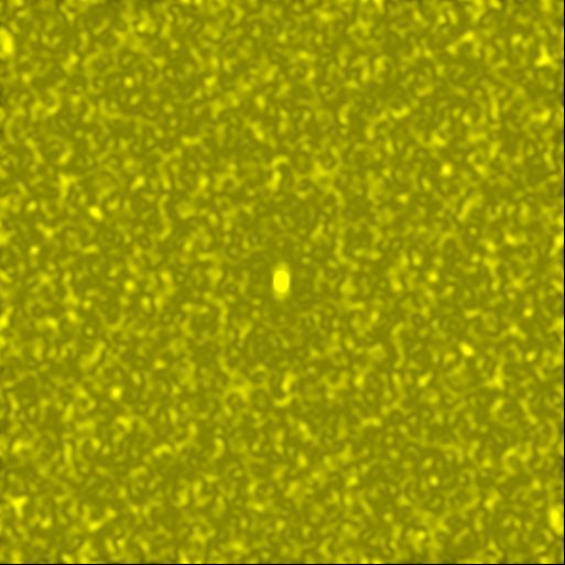
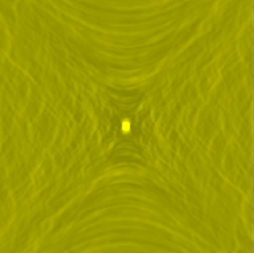
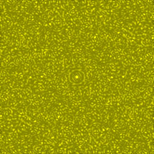
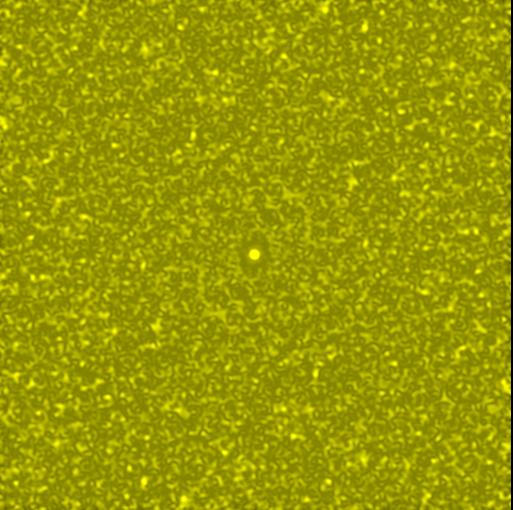
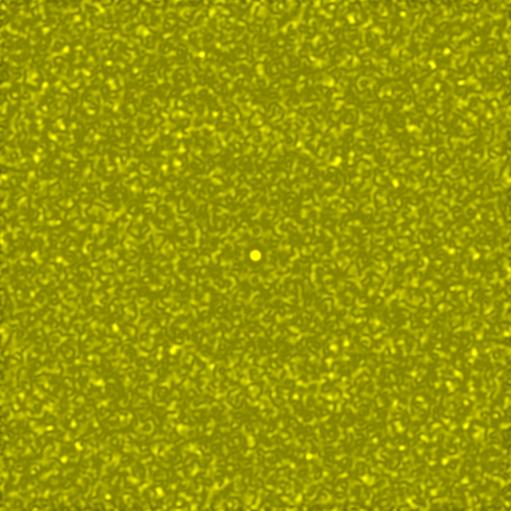
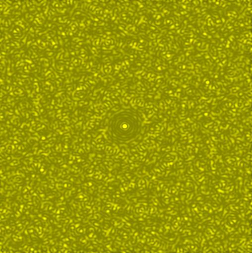
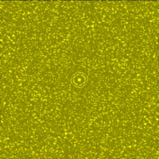
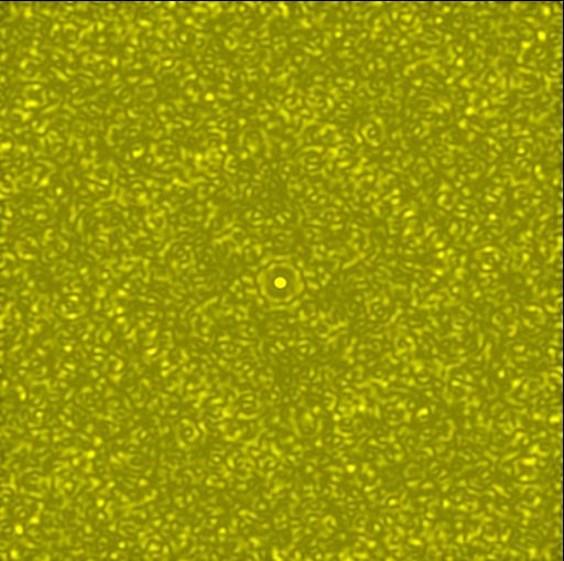
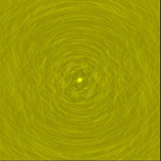
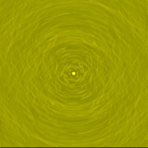
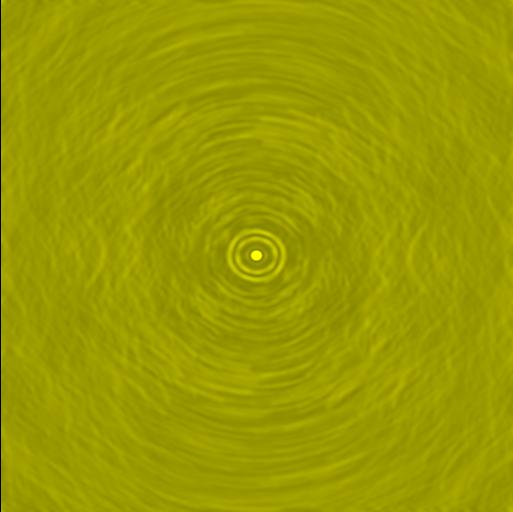
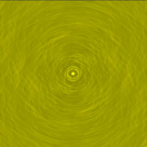
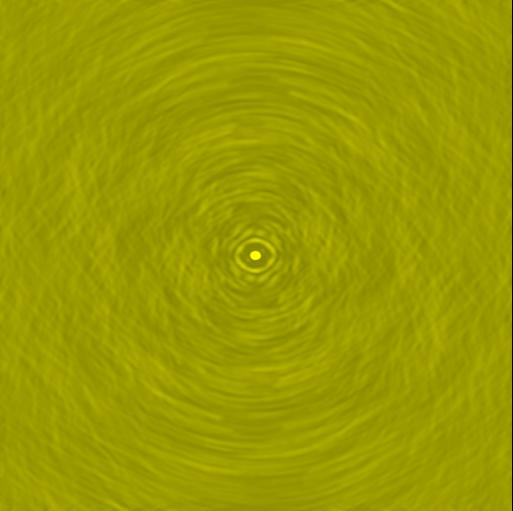
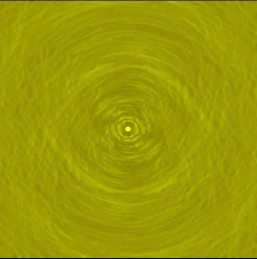
Fig 12. Left: Plot of the 4 hour B-array zoom spiral beam for a declination
-23 source. Plotted between 0 and 3%. Right: Contribution to the
dirty beam from the 3.9% of uv points which lie beyond the
outer radius of the dual ring uv coverage, also plotted in the range 0 to
3%. The rings in the centre
are an artifact of taking a sharp uv cutoff. The largest far sidelobe
contributed by the outer uv points is 0.5%
4.4 Long track dirty beams
Below we compare the long track dirty beams for the zoom spiral
and dual ring arrays. The main difference between them is that
the latter has ring-like near-in sidelobes which the zoom
spiral does not have. This causes a significant
difference in peak sidelobes with 20 beams between the two arrays
(see Table 3). On average the peak sidelobes of the zoom array
are only 59% of the peak sidelobes for the dual ring. In addition
the peak zoom array sidelobe occurs on a distant peak whereas the
peak sidelobe for the ring array occurs a part of a coherent
structure with many adjacent parts of the beam having almost the
same value. The reason for the much larger
near-in sidelobes in the case of the dual ring is the 'stepped'
or 'wedding cake' nature of the uv uv coverage, while the uv
coverage density distribution for the spiral is close to gaussian
for all arrays other than A. Another useful way to look at the long track
dirty beam is as a superposition of rotated and EW-stretched
snapshot dirty beams. We can therefore see that although distant
sidelobes are decreased in going from snapshots to long tracks
near-in sidelobes will be hardly decreased at all.
| |
A-Array |
B-Array |
C-Array |
D-Array |
| Zoom Spiral |
|
|
|
|
| Double Ring |
|
|
|
|
Fig 13. Long track (4hr) beams for a source at declination
-23 degree, Top row, zoom spiral. Bottom row
double ring designs. From left to right beams for
arrays A-E or equivalents are shown
The plotted grayscale ranges between -5% and +10%.
| Array |
Zoom |
Ring |
Ratio Zoom/Ring |
| A |
0.0259 |
0.0427 |
0.60 |
| B |
0.0215 |
0.0385 |
0.55 |
| C |
0.0276 |
0.0469 |
0.58 |
| D |
0.0246 |
0.0385 |
0.63 |
Table 2. Peak sidelobes within a radius of 20 beam FWHMs
for a 4 hour long synthesis of a declination -23 deg source,
for the zoom and ring arrays respectively.
Below we show North-South slices through the dirty
beams for the spiral and double ring arrays respectively.
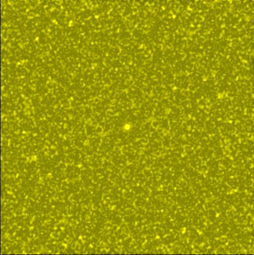
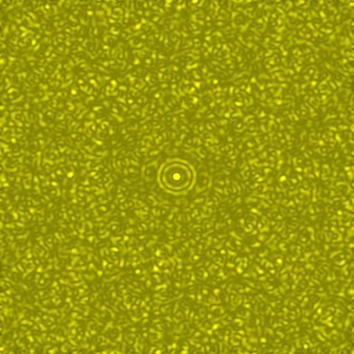
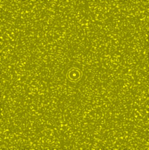
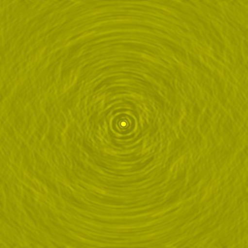
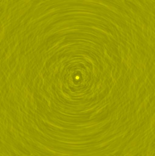
Fig 14 Left: A North-South slice through the B-array zoom spiral
dirty beam. Right: A North-South slice through the B-array
dual ring dirty beam.
4.5 Imaging Simulations
Both the ring and zoom arrays have been tested imaging a series
of test images. The results of these CLEAN simulations can be found
at
Heddles Simulation Page.
Although
in some cases the ring strawperson gives better reconstruction, in general
the quality of the zoom array constructions are slightly better expecially
for long tracks. Usually at given brightness level in image the rms
reconstruction errors are about a factor of 1.5 to 2 less. For B-array
in particular the fidelity index metric
in some cases gives a different result; implying
a few (100 pixels is 4 beams) regions of very high fidelity index . It is
unclear why this is difference between the the two methods of measuring
image quality. Possibly when one adds both errors at a bright point to
bowl like negative errors the value of the parameter
(model/error) can have fortuitously large values
at a few isolated points.
5. Comparisons with Double Ring Array: Operational
and other considerations
In this section we consider other aspects of array design other
than uv coverage and beam which can be considered operational
or practical matters; and compare the zoom and dual ring
array concepts for the intermediate configurations.
5.1 Array Flexibility
One of the most attractive features of the zoom array is
that it is a very flexible design. In this memo we have
concentrated on configurations of the spiral array in five
nominal configurations which match in resolution
configurations offered by the dual ring arrays. Note
that this has been been done to facilitate
inter-comparisons between the two array styles; it does not
imply that the array is restricted to these configurations.
The zoom array could in contrast to the the dual ring
instead operate at say three fixed resolutions
or seven, or whatever, with the choice of resolution being made after
construction in response to the types of science that are popular in
the 2010s or 2020s. For instance if line ratio imaging between particular
molecular transitions became popular that could easily be accommodated. Note
that the total number of antenna moves that must be made to accommodate
different numbers of configurations is constant. Antennas are always
moved from the outside pads to the inside pads and after making 126
antenna moves we will have moved all antennas from the largest to
the most compact configuration. All that changes when we go to a smaller
or larger number of configurations is whether antennas are moved in
short of long 'bursts'.
At one extreme the zoom array also allows the possibility of gradually and
smoothly changing the resolution of the array by for instance moving
three antennas every four days or so. This approach has certain astronomical
advantages in that all resolutions are offered removing the need
to lose sensitivity by tapering. This approach also has operational
advantages in that a small crew can be employed continuously for antenna
moves which can then all be accomplished in the morning before
winds get high. The array should also be more resilient to delays in
moving antennas due to weather . The astronomical efficency and operational
aspects are discussed in detail in Conway (2000) memo 283 and are
further discussed in the section below.
The zoom array no matter whether operated in burst or continuous
reconfiguration mode is more flexible in another sense as well.
Essentially it just comprises as 1/r^{2} pad density distribution
without any in-built scales. This allows a great flexibility
in how the pads are populated in any given configuration. This
population scheme can be changed in response to observing
experience just like the case of the VLA where C-array was recently
altered to allow more short spacings. The zoom array probably gives
more flexibility in this regard than the dual ring in which all
antennas must be placed on a limited number of concentric rings.
5.2 Operational Issues
Both the zoom spiral and dual ring arrays have virtually the same
number of antenna pads (195 for the spiral and 192 for the
ring) and require virtually the same number of moves to go through
all configurations smaller than 3km (126 for the zoom spiral
and 128 for the dual ring). What potentially is different is the
order and tempo of how the antennas are moved during a reconfiguration
cycle. When considering the operation of the zoom array it is useful
to consider two possible operation plans namely 'burst' and
'continuous'.
'Burst' reconfiguration - In this mode
the zoom operates just like the dual ring array with fast
reconfiguration between a set of fixed resolution arrays. We
will we assume that just like the strawperson dual ring design
the zoom operates in 5 array size smaller than 3km (although of
course the number can be varied for the zoom). In this case every
year we can spend two periods of 4 weeks
in each array size (A,B,C,D,E). It could take perhaps 4 days to reconfigure
between configurations (assuming we move 8 antennas per day)
North-South elongated 'hybrid' configurations can be accommodated
(see Section 3.3) in two possible ways. If only a small amount of hybrid
time was requested by astronomers we would simply move the eastern and
western most antennas first during the 4 day move period and slot
observations in once antennas had calibrated baselines. If much more
hybrid time was requested we could break the reconfiguration into
two halves. In the first half the 16 easternmost and westernmost
antennas would be moved, taking two days to reconfigure, giving the
North-South hybrid. Perhaps a week would be spent in the hybrid
configuration plus two more days reconfiguring. In this mode of course
only 3 weeks could be spent in the the full configurations (A,B,C,D and
E). In addition to all of this there would be one period per year
of perhaps 4 weeks in the 12km configuration.
'Continuous' reconfiguration - In this mode
the array is reconfigured slowly but almost continuously. Because
of the need to calibrate antenna pointing before a moved antenna
can join the array (and the need to determine sub-wavelength
accuracy baselines - although this can in principle be
partly done later and the corrections added to the correlated data)
it is probably not efficient to move less than than 3 or 4 antennas
at once. In Conway 2000a (memo 283)
a scheme was proposed to move 3 antennas
twice a week, on Mondays and Thursdays. On average then a
complete cycle through all the configurations smaller than 3km
(126 moves) would take 21 weeks. Two full cycles could be
accommodated per year, adding 2 extra weeks twice a year
'stopped' in each of A and E arrays. Finally there would 6 weeks
per year in the 12km array (including move time)
scheduled once a year. The overall cycle structure is indicated in
the figure below.
During the continuously reconfiguring
part of the cycle, the Monday and Thursday moves could for instance
accommodated by 3 transporters and three crews taking 1 - 2 hours
to do the move, and all moves completed by 9am or 10am local
time. A crew of 6 would be used for reconfiguration. On other
days when not reconfiguring these personnel would be used for
antenna maintenence. There would in the suggested cycling scheme
be three long moves per year when all transporters (5?) and all
available staff used to moves antennas as quickly as possible. These
'long moves' could comprise the moves to and from the 12km array and
from the E to A array.
During the main periods of continuous reconfiguration there will
be occasional Mondays and Thursdays
when a reconfiguration is not possible due to
high winds or snow. In this case the reconfiguration can be attempted
on one of the two or three following days that otherwise would be
allocated to antenna and receiver
maintainence. If these days were also effected by weather
we could try to attempt two configurations per crew on the
next scheduled reconfiguration day and so on. In the scheme
suggested below the array would be reconfigured inwards starting
with A array and shrinking the array to E array. This means that
if a reconfiguration was missed the scheduled astronomical
observation would go ahead, but with a resolution that is 7%
larger than originally scheduled. By gaussian tapering the
data the desired resolution can be recovered with a loss
of only 2% in sensitivity (see Conway 2000a, memo 283).
Hybrid arrays can be incorporated into continuous
reconfiguration in two possible ways. In the first method
for 5 reconfiguration days (2.5 weeks) the Eastern most and
Western most antennas are preferentially moved inward and then for the
next 5 reconfiguration days (2.5 weeks) the Northernmost and Southernmost
antennas are moved. For most of the 5 week period the beam
would be fairly round (and a perfectly round beam can be recovered
with little sensitivity loss by suitable tapering), but in the
middle of this period the array would be extended North-South
with good uv coverage and near circular beams for sources
as far north as declination 30 degrees. In the second
method we could move inwards through the arrays keeping circular
symmetry twice a year and outward through the configurations
once per year this time filling antenna pads within an elliptical
area.
A possible phasing of the
reconfiguration cycle with respect to season is also given in the
figure below (this is only a first suggestion).
Amongst the issues to be considered in deciding the phasing is the desire
for both high resolution (A) and compact (E) array observations
to have the high phase stability, high opacity winter weather, and the
operational desire to move to and from the 12km array during
the least windy months (say November and December).
Fig 15. A possible reconfiguration scheme for ALMA using
continuous reconfiguration. Click for higher resolution.
In comparing the operational aspects of running the zoom spiral
with the dual ring strawperson we can distinguish between generic
advantages inherent in the array geometry and the
advantages of using continuous reconfiguration.
Generic Advantages
One important difference between the two
arrays is that however the zoom is reconfigured (either via
conventional bursts or continuously) it is always left in a
self-similar configuration - so the uv coverage is always smooth
with a good beam pattern. This is in contrast to the dual ring
array - if bad weather hits at the start or end of a 'burst'
reconfiguration period then antennas can be left 'stranded' on
either the inner or outer ring. The uv coverage of an array with
only 2 or 3 antennas on the outer ring will not be particularly
good and the data from these antennas will in practice often
be deleted. Note that the wind limit for
observing (at low frequency) is less than that for moving
antennas. Consider also the scenario that reconfiguration starts
in the morning but winds rise during the day and reconfiguration
must be abandoned. The winds will die down again in the evening
and observations can begin again, but it will be dangerous and
undesirable to reconfigure during evening/nighttime. The array
will then have as much as 16 hours of observing time (often
of excellent quality) in a non-optimum configuration.
Advantages of continuous reconfiguration Some of the
advantages of continuous reconfiguration, such as a permanently
employed crew at the site, and the ability to do all reconfigurations
early in the day before winds rise have already been mentioned.
There are also astronomical advantages in that resolutions
in different line transitions can be matched without losing
sensitivity due to tapering.
It can also be argued that continuous reconfiguration
is more robust to weather related problems. In the case
of conventional burst reconfiguration if a period of bad weather
lasting say a week hits during the scheduled reconfiguration
period the whole cycle of configurations can be effected. Instead
of 4 weeks in the next configuration only 3 weeks will be possible, and
a significant number of projects will have to be delayed six months
or observed in configuration a factor of 2 different in resolution
to that requested. More seriously the schedules of the personnel
involved in reconfiguration have to be changed, and the whole large
crew put 'on standby' until daytime weather is good again. It can
of course be counter-argued that with continuous reconfiguration we
are also virtually certain to lose some reconfiguration days
due to weather also. However is surely best to share and dilute
the risk rather than concentrating it into a few big moves. An
analogy can made that most of us choose to insure their car and have
a 100% chance of losing $500 per year rather than a 1% chance of
losing $50,000.
5.3 Hybrid Arrays
As shown in Section 3.3
the zoom array geometry can easily accommodate
North-South elongated hybrid arrays for looking at far Northern
or far Southern sources.
The resulting uv coverages are smooth,
the resulting dirty beams have no large sidelobes, and are close
to circular for sources for declinations up to +30.
Note that the total number of moves required to
go through all array configurations stays the same whether or
not one uses hybrid arrays or not.
Although an example was only shown for a B/C hybrid, similar
hybrids are possible for all arrays. This includes the possibility
of a D/E hybrid which is particularly useful because of the high
degree of shadowing that occurs in E array for observations of far
Northern or Southern sources. No comparable plots of beam shapes or
uv coverages have yet been produced for the dual ring arrays to
directly compare. For this design hybrid arrays would be produced by
moving the Eastern or Western most antenna in the outer ring first.
Since the ratio of radii of the rings is approximately 2 it
is unclear whether the resulting uv coverage will be good.
5.4 Fitting the array into the Site.
In a recent memo Butler and Radford (2000, Memo 338)
have identified a number of places which are suitable from the point
of view of smoothness and flatness for placing the centre of
the array. They have also investigated positions identified
in the strawperson designs.
Note that the zoom array design described in this
memo ('zoom2') has exactly the same centre as the
strawperson dual ring array produced by Yun and Kogan (2000, memo 320).
This was done deliberately to facilitate comparison between the
two design styles, it did not necessarily imply that this
was the best place to centre the array. In the memo of
Butler and Radford the position which is discussed as
'spiral centre' in the position identified in the 'zoom1'
design (Conway 2000c, memo 292), not the one used in this memo. In any
case both centres were found to be less than optimum from a site
point of view.
The site identified by Butler and Radford
as 'Chanjnantor Best' is difficult
to use for any design which
has a high degree of pad sharing because it lies right at the edge
of the 3km flat area at Chanjnantor. The second best site which
is near the NRAO containers however
is a possible candidate, since it lies halfway between the centre
of the 3km flat area and its perimeter. Experiments with zoom arrays
with an offset centres at this place show that relatively little
distortion or 'squint' is introduced into the dirty beam and that the
uv coverages remain quite good. A preliminary offset design
will be presented very soon in a separate memo,
(a preview of work in progress can be found at
Offset Zoom Array . )
For some reason there is a perception that it is harder to
fit a zoom design into the site than a dual ring design, but
this is not true. Considering
non-offset concentric arrays it is clear that once the largest
array size and the resolution step between rings is defined there are only
two overall degrees of freedom (plus local distortion)
in placing the array into the site, namely
the x and y coordinates of the array centre. In contrast for a
zoom spiral design the array can be rotated to avoid obstacles
without changing the circular symmetry of the uv coverage. In addition
one can choose either clockwise and counter-clockwise designs
and can vary somewhat the pitch of the spiral arms to avoid
obstacles.
5.5 Roads and Conduits.
A detailed road and conduit plan has not yet been
made, however sketches suggest pads can be connected
in the zoom array using 5 branch roads radiating from the centre,
and curving to avoid quabradas, with additional
'twig' access roads to the pads. The pads on the outer
ring would also be partly connected together where the terrain
allows it. A sketch suggests a total road/conduit length
for the smaller than 3km arrays of about 19km for the zoom. For
the dual ring arrays connecting all the circles together takes
17.5km, plus two radial access roads adds another 3km, giving
20km. The total length of roads and conduits is likely
in practice to be very similar for both styles of arrays.
5.6 Combined Array Imaging
For the most complex sources it is clear that data from several
configurations must be combined to achieve the best imaging. This
should cause no special problems for the zoom array. The uv density
distribution of a single configuration is gaussian shaped (see Figure 7),
with a flat top at intermediate to short baselines and then
a hole in the centre of the uv plane which is approximately
1/40 or 1/50 of the longest baseline. The distribution
differs significantly from the VLA which is not flat topped
but is power law until a sharp cutoff at small baselines;this
peaked uv density makes combining arrays more difficult.
To fill in the hole in the centre of a single configuration
spiral uv coverage a snapshot in an array two or three sizes smaller
should be added. For instance to B array could be added to D array
observations. To obtain a smooth uv density distribution at the centre
of the uv plane the integration time of the D array snapshot
need only be 1/2.1^{4} or 1/20 that of the B-array; or 12 minutes in
D array for a 4 hour long track in B-array. To make the inner parts
of the combined uv density density smooth it may be necessary to re-weight
the D-array data losing some sensitivity but this loss is easily made
up by integrating two or three time longer in D array. Finally after
using them to cross amplitude calibrate the two configurations it might
be desirable to delete the shorter baselines of B array, since the uv
plane filling due to these baselines is much more ragged than the
overlapping smooth uv coverage due to the smooth D array snapshot.
Because a relatively small fraction of the B array uv data is
effected (10% -20%) the loss in sensitivity due to doing this
re-weighting will be small.
It is not envisioned that there will be any significant difference
in combined configuration performance between dual ring and
zoom spiral designs, because to first order the uv point density
distributions are so similar.
5.7 Mosaicing
Testing the performance of the candidate designs in mosaicing
mode has been limited to date by the lack of available software.
Again given the similar uv density distributions of the two
candidate array designs it would not be expected that there
would be a large difference in performance. In particular
both styles of array have exactly the same design for E-array.
For D array both designs fully occupy the 150m diameter ring
giving the same number of very short baselines going down to
a fraction of an array diameter.
5.8 Pointing Errors
One of the factors that will limit the quality of ALMA Images
at intermediate and high frequencies will be the effects
of pointing errors. These have been simulated by Kogan(2000)
(memo 317) and Morita (private communication). Again given the
similar radial uv distributions we expect the zoom and ring
arrays will have a similar response with respect to pointing
errors.
It has been noted that pointing errors can limit
the advantage of an array with better imaging performance. It should
be noted however that the likely limitation in fidelity due to
pointing errors is a strong function of both the source structure
and the observing frequency. At 230GHz assuming a pointing
error rms of 0.6'' and using an image consisting of equally bright
regions scattered over the primary beam Morita found that on-source
fidelities for a spiral array were reduced from about 100
(with no pointing errors) to 75. Hence although significant
the effects of pointing error were not dominant. The tested
array still performed significantly better than another test
array (a simple single ring array). The contribution
of pointing to amplitude errors will scale quadratically with
frequency for bright regions at the centre of the beam
while it will be linear for regions near the half power point.
For isolated sources with their brightest points in the centres
of the beam and/or observations below 115GHz there will be many
cases where pointing error effects are smaller than those
due to uv coverage effects. Although the computing requirements
are immense it is also possible that the antenna based pointing
offsets can be solved for as part of the imaging process.
5.9 Phase Noise
In a separate memo we consider the phase noise effects in the
image domain for two arrays with the same resolution but
different degrees of central concentration. In the case that
all baselines in a configuration are smaller than the thickness
of the turbulent layer (often 500m at the ALMA site, Robson 2001,
Memo 345)
then rms phase error are proportional to r^(5/6) where r is the
baseline length, for longer baselines rms phase errors are instead
proportional to r^(1/3). We assume the worst case that we apply
phase correction (e.g total power monitoring) and the corrected
phase errors have the same dependence on baseline length but
with the amplitude of the phase errors being scaled down. This
would occur for instance if there were an error in the derived
scaling factor between the atmospheric phase and the total power.
In the case of observing a point source in the small baseline
regime we show that phase error image errors are proportional to the
r^{10/6} moment of the array baseline length histogram. The
resolution of an array depends on the second (r^2) moment of the same
histogram, hence in this regime two arrays with the same
resolution but different degrees of central concentration have virtually
the same image phase errors (with a slight advantage to the
more condensed array). If the source is resolved then the
phase noise due to short baselines dominates more. These short baselines
have smaller phase noise compared to longer ones; therefore out of
two arrays with the same resolution the more concentrated one
with more short baselines will have smaller phase noise. Similarly
if we consider configurations in which many of the baselines
are longer than the atmospheric turbulence thickness r_{o} the more
concentrated array again has lower phase noise errors even for
a point source. We can see this because all baselines
longer than r_{o} contribute virtually the same phase
noise but baselines with r less than r{o} have a rapidly decreasing
phase noise contribution with r. Between two configurations with the
same resolution, the more centrally concentrated one will therefore
have less phase noise. The above arguments lead to a
counter-intuitive result, that between two arrays with the
same resolution the one which has a longer maximum baseline can have
lower phase noise. The reason is that if an array has a small
percentage of distant uv points then to give the same resolution
it must also must have significantly more short baselines which
more than compensate.
5.10 Tapering.
It is often useful to reduce the resolution of an array
by increasing the weight of the short baselines. This procedure
compared to natural weighting always increases the noise per beam;
however the signal to noise to diffuse low brightness temperature
emission can be increased by this procedure. Figure 9 of Conway 2000a
(memo 283)
shows how the loss in sensitivity in terms of increased
mJy/beam changes as the array is gaussian weighted to give a
larger beam. The noise only increases gradually with tapering,
and reached an increase of factor of 1.13 once the beam is
tapered to give 1.4 times larger beam size
Given their similar
radial uv density distributions only minor differences are expected
between zoom and ring array styles for loss of sensitivity as a
function of tapering. However it is expected that the
zoom array will be slightly more efficient since it is slightly
more concentrated, as has been borne out by simulations.
5.11 Inverse Tapering and Super-resolution
To increase the resolution
of existing arrays uniform weighting is often applied. This
is a fairly crude procedure which looks at the local density of the
uv coverage (i.e. uv points per uvcell) and weights inversely according
to the occupancy. This procedure is very useful for the case of VLA
data where it reduces the effects of the spikes
in the uv coverage due to the intra-arm baselines.
When applied to the fairly smooth radial uv coverages of the zoom and ring
arrays it is less successful (there is a sharp transition in weighting
at a uv radius where the cell occupancy becomes greater than 2). For
both array styles significantly increased sidelobe levels result. A more
logical way to increase resolution is to instead apply
global radial weighting methods which emphasise the longer
baselines. Seeing the problem from constrained optimisation point of view
it is possible to work out the optimal weighting as a function of uv
radius for a given beam size (i.e. a fixed weighted
mean square baseline length) which minimises sensitivity loss.
It is well known that
in addition to applying uv re-weighting to increase resolution
it is also possible to choose a somewhat smaller CLEAN restoring
beam. CLEAN or other deconvolution algorithms extrapolate
the uv data to larger uv radii than those measured. This extrapolation
is always limited in quality and we convolve with a restoring beam
to reduce its effect in the final map. In a sense
the step of using the clean beam can be thought of as regularising
the problem to answer the question of what the sky would look
like if it was first convolved with a particular restoring beam
before being observed.
The Fourier transform of the CLEAN beam restored image
certainly equals the uv coverage that would have been obtained from a
hypothetical source which was convolved with the restoring beam before
being observed. Seen in this way the choice of the size of a CLEAN
beam can be seen as a fairly arbitrary step. No simulations have yet
been performed comparing the performance of the two array styles
with super-resolved CLEAN beams, but since the zoom spiral baselines
extend to larger uv radius in a given configuration
it is probable that the super-resolution performance of the zoom might be
slightly better.
6. Summary
In this memo we have presented a strawperson zoom array design
and compared it properties to the competing dual ring array
design. We argue that compared to the competing array the zoom
has a number of advantages.
1. Imaging Quality
As discussed in Section 4 the
peak dirty beam sidelobe level for snapshots is comparable for the
two designs but for long tracks the zooms' sidelobe
peak is 60% of the level
for the ring. The radial uv distributions are smoother for the
spiral with less clear holes. The uvcell filling factor is comparable
with the spirals filling factor being slightly smaller for snapshots
and slightly larger for long tracks. The present spiral designs have
a wider range of baselines compared to the ring. CLEAN Imaging simulations
appear to show a trend of somewhat higher dynamic range (by a factor
of 2) for the spiral than the ring. Although pointing errors will
eliminate differences in imaging quality in some cases; in other
cases (e.g 115Ghz observations of isolated sources) imaging quality
differences will remain an issue.
2. Flexibility The zoom is a very flexible array and can
be operated in a wide number of different modes. It can be operated
as a set of fixed configurations with the number and resolution of
the configurations being adjustable. It also has the option of being run
as a continuously reconfiguring array, which has certain operational
and astronomical advantages. The mode of operation for the zoom can be
changed easily after construction in response to changing scientific
demands once the array is in operation. Finally there is more
flexibility in the choice of pad occupation schemes than is the case
for the dual ring.
3. Hybrid Arrays The zoom geometry has demonstrated excellent
uv coverages and beams when in North-South elongated hybrid arrays
suitable for observing far North or far South sources. No extra pads
need be built to accommodate a hybrid D/E configuration which is
needed to avoid shadowing for observing Northern hemisphere sources.
Unfortunately no similar hybrid configurations have yet been presented
for the dual ring design to allow a direct comparison to be
made.
4. No Stranded Antennas
Whether operated in 'burst' or
'continuous' reconfiguration mode; after making an antenna move
the array is always left in a self-similar pattern, all that changes
is the resolution. In contrast for the dual ring if reconfiguration
must be interrupted due to weather reasons there can be a few
antennas 'stranded' on the outer ring, giving poor uv coverage,
whose data would in practice often be deleted.
5. Lower Phase Noise
In the case of observing point sources in the small array limit both
array styles are expected to have the same image phase noise
after doing total power phase correction. However for observations
of resolved sources and/or observations with configurations with
baselines longer than the thickness of the turbulent layer the zoom
array has an advantage. This arises because the zoom is a slightly
more centrally condensed array. Counter-intuitively the zoom
can have lower phase noise even though it has larger maximum baselines
than the dual ring.
6 Offset Centre Designs
Offset centre zoom array designs with the most densely packed
parts to the array close to one of the sites identified by
Radford and Butler as flat and smooth have been produced
(see
Offset Zoom Array . ). The beam shapes and uv coverages
remain of high quality. No similar design has yet been produced
for the dual ring concept. Because its antenna pattern is smoothly
increasing in density with decreasing radius there are reasons to
believe that such offset designs would give better uv coverage and
beams than dual ring designs.
All the above points depend on the zoom array geometry and not on
how it operated (i.e. 'burst' or 'continuous' reconfiguration) in
addition there are some extra advantages that the zoom has
if operated in continuous reconfiguration mode.
7. Matched Resolution and High Observing Efficiency
Continuous reconfiguration mode allows observations in different
line transitions to have exactly matched resolution. Because the
need to taper the data is reduced the observing efficiency (i.e.
total used observing baseline hours) is maximised.
8. Operational Advantages A small crew can be permanently
employed doing reconfiguration, rather than requiring intermittent
large amounts of personnel to execute big moves. All reconfigurations
can be made in the mornings before (winter) winds get too large.
This mode 'spreads the risk' of the impact of weather related
reconfiguration delays compared to one in which infrequent big
moves are made; minimising impact on personnel schedules.
Point 7 is probably
less than compelling than point 8, and the
choice between 'burst' and 'continuous' reconfiguration modes will
and should be determined by operational concerns.
After starting from quite different positions
the two proposed designs have converged quite
considerably. The ring design is now a set of five concentric circles
each different by a factor of 2.1 apart in size, the outer two of which
are occupied at any one time. The zoom array can be considered as a
much larger number of concentric circles of antennas with many more
outer circles occupied simultaneously. The dual ring is in effect
itself a 'zoom'
array except that it only zooms over fixed scales of 2.1. Given the
convergence that has occurred it is not surprising that there are no
highly dramatic differences between the two array designs. However
in each of the eight points above the zoom array seems to have an
advantage. There seems in contrast to be no compelling reasons
to built in fixed scales into an array when a scale free array
exists - these fixed scales simply reduce flexibility and add
inhomogeneities into the uv point radial distribution. The
only justification for placing antennas on rings is to improve
the coverage of the very shortest baselines, but we have shown
by suitably populating that the pads the zoom array can actually
have better short baseline coverage than the dual ring arrays
(see Table 1 and Figure 7).
7. Future Work
Future work should focus on producing a detailed site
plan. At the next level of complexity plans for roads
and conduits should be built in. The next iteration of the design
should also probably allow smaller baselines. The dual ring arrays
have ratios of maximum to minimum baseline lengths of order 40. The
zoom configurations have ratios of between 40 and 70. In comparison
the VLA with 2.4 times fewer antennas has a ratio of 45 in its non-hybrid
arrays. Modifying the zoom array to allow baselines down to 30m in
A array and 15m in B-array might be desirable. Another area which
requires more work is the 12km array and the interface with the present
A-array. Site restrictions mean that the 12km array must be a ring,
in which case its resolution will be more than 4 times larger
than the present A-arrays which are still somewhat
centrally concentrated (the resolution ratio will be closer
to 5). In the zoom design by adding about 16 pads to the
present A-Array design, so that virtually all antennas could be put
around the perimeter of the 3km area, an A+ configuration with 30% higher
resolution than the present A could be produced. Such an array
would help bridge the gap to the 12km array.
The new designs must be optimised, and its not clear we have the
best tools yet for this optimisation. It seems that
there are strong indications that optimising the beam shape is the
best way to ensure imaging quality. Elaborations of the
Kogan algorithms that optimise the image sidelobes for
observing gaussians of all angular sizes is one possible approach,
This metric incorporates beam quality and range of baseline
length sampled into one single metric.