 |
ABSTRACT
A first attempt is made to fit a zoom spiral geometry into the
terrain at the Chajnantor site. The objectives were to obtain
a first order estimate of how terrain effected uv coverage, and to
locate possible sites for the most compact part of the array. Only manual
adjustments to the antenna positions were made. No attempts
have yet been made to optimise for uv coverage, despite this
it appears that such an array can be fitted into the terrain
while preserving good uv coverage. One possible position
for placing the most densely packed part of the array is
identified. This region is on a slope with mean gradients
of about 3 degrees. Further investigations of the geology in
this region are required to see how suitable it is for building
antenna foundations. The tradeoffs between ease of operations,
uv coverage and the maximum gradients at which the the antenna
transporter must operate should be carefully considered.
1. INTRODUCTION
This memo describes a first attempt at fitting a spiral zoom
array into the terrain at the Chajnantor site. The objectives
were (i) to determine possible sites for the array
centre and (ii) get a first order estimate of how the uv
coverage degrades when taking terrain into account.
The procedure was simply to take a spiral
array similar to the one presented in Memo 283 and
manually rotate and shift it to avoid bad terrain
features. The remaining antennas which lay in difficult
terrain were then moved slightly, again manually, without
any consideration for optimisation of uv coverage.
The next step would be to optimise the array in some way. This
could be done by minimising uv coverage and/or beam metrics.
Promising results have been obtained in reducing the peak
sidelobes of spirals using the beam sidelobe minimisation program
of Kogan (AIPS task CONFI, see Memos
226, 247 etc). Without terrain
constraints this optimisation reduced peak sidelobes in the
snapshot beam by a factor or 2 or so. The next step would be
to run the sideblobe minimisation program incorporating a
terrain mask constraint.
|
|
2. ARRAY DETAILS
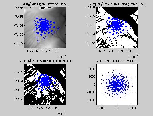
The manually fitted array is shown in the figures. As described in
Section 1 the antenna pads were only placed at positions
allowed by a terrain mask. The mask used (Fig 1, bottom left)
incorporated a limiting gradient of 5 degrees (on a scale of order
10m as set by the pixels in the digital elevation model). This
mask has been generated by B.Butler (NRAO). A 5 degree gradient
limit is a somewhat arbitary choice, but is probably a good
starting point. It is thought that gradients much larger than
5 degrees would probably be hard to deal with without making
antenna move operations difficult and the antenna transporter
expensive (though no detailed cost-benifit analysis have
been done).
Figures 2,3,4 show the array superimposed on the 5 degree elevation
mask at different scales a factor of 2 apart. These figures show
the main part of the array which is constructed from antennas
on 3 tightly wound spiral arms, with 48 pads per spiral arm.
Unlike in previous memos the lines tracing the three 'conceptual'
spiral arms have not been plotted; this and the fact that some
antennas have been moved to avoid terrain features are the main reasons
the the arrays' spiral structure may not be immediately obvious.
As described in Conway (1998, 2000) [Memos 216, 283] the resolution
can be gradually changed by movng antennas at the ends of the spiral
arms to unoccupied pads at the centre (the 'zoom' property).
Note that three of the Northernmost most
antennas in the spiral (see Figures 3 and 4)
have been shifted slightly South to avoid coming within 500m of the gas
pipeline which is the currently agreed constraint. The zenith
snapshot uv coverage in Fig 1 (bottom right) is calculated assuming
the pads 28 to 48 on each of the spiral arms are all occupied.
This plot shows that the antenna position perturbations introduced to
avoid the gas pipeline and terrain do not effect the uv coverage
very much.
3. LOCATION OF THE ARRAY CENTRE
The array shown in the figures is centred
at Easting - 628590m, Northing - 7454000m. This position is
about 1km East of the MMA container, and from a quick look
appeared to be the best as far as
flatness and avoiding arroyos etc was concerned; while being
consistent with choosing a site close to the centre of the available
area. Figure 5 shows a
contour map at the array centre. The 'dense pack' part of the
uv coverage lies (see Figure 5) on a gently sloping part of the
terrain with mean gradients of about 3 degrees. The position of the chosen
centre is a bit north or the centre of the overall Reuleaux triangle
(see Figure 1), but
this doesn't seem to effect the uv coverage very much (see Figure 1, bottom
left). It would be very interesting to know more about
the geological conditions
at this part of site, and know whether this region is suitable
for building antenna foundations. It is also very important to know
whether the mean gradients found in this region are compatible
with the envisioned transporter and operational specifications. A
number of other possible array centres are possible if the one
chosen does not prove suitable, however from the point of view
of uv coverage on a zoom array it is desirable to have the most
compact part of the array situated within about 1km of the centre
of the overall available area. Given this there may be tradeoffs
to be made between situating the dense pack part of the array
on the flattest terrain and having good uv coverage and the
ability to zoom.
Fig 2. Array superimposed on 5 degree local gradient mask (click
for more details). Filled
symbols are occupied pads and open symbols unoccupied pads.
Fig 3. As Figure 2 but zoomed by a factor of 2 to show centre of array.
(Cick for more detail).
Fig 4. As Figure 2 but zoomed by a factor of 4 to show centre of array.
(Click for more detail)
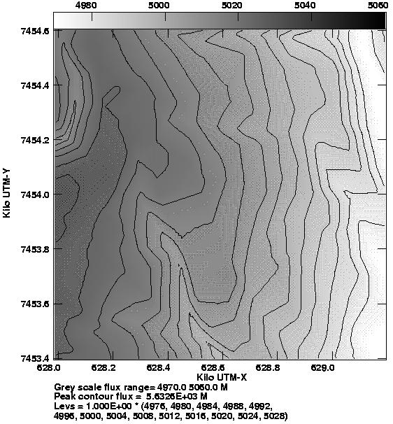
Fig 5. Contour map/grayscale showing terrain details in region of
the array centre. Area plotted is the same as that plotted in Figure 4.
(click for more detail).
APPENDIX - Software
The MATLAB v5.1 files used in this memo for displaying the array and terrain
can be found at http://www.oso.chalmers.se/~jconway/ALMA/SOFTWARE/MATLAB/SPIRAL12
.